library(gamlss)
library(gamlss.ggplots)
library(ggplot2)1: Distributional Regression Models
Dutch boys BMI for boys aged between 10 and 20 years
We use the Dutch boys BMI data to illustrate the regression concepts discussed in Chapter 1. The dataset dbbmi is in the gamlss.data package.
Data and model setup
Load the dbbmi dataset, create the subset of boys aged 10 to 20 years, and compute the linear model.
data(dbbmi)
# data for boys aged 10 to 20
db_bmi_10 <- dbbmi[db$age>10&db$age<20,]
# linear model
m1 <- gamlss(bmi~age, data=db_bmi_10, trace=FALSE)
summary(m1)
******************************************************************
Family: c("NO", "Normal")
Call: gamlss(formula = bmi ~ age, data = db_bmi_10, trace = FALSE)
Fitting method: RS()
------------------------------------------------------------------
Mu link function: identity
Mu Coefficients:
Estimate Std. Error t value Pr(>|t|)
(Intercept) 10.66377 0.25033 42.60 <2e-16 ***
age 0.59348 0.01693 35.05 <2e-16 ***
---
Signif. codes: 0 '***' 0.001 '**' 0.01 '*' 0.05 '.' 0.1 ' ' 1
------------------------------------------------------------------
Sigma link function: log
Sigma Coefficients:
Estimate Std. Error t value Pr(>|t|)
(Intercept) 0.90740 0.01217 74.56 <2e-16 ***
---
Signif. codes: 0 '***' 0.001 '**' 0.01 '*' 0.05 '.' 0.1 ' ' 1
------------------------------------------------------------------
No. of observations in the fit: 3376
Degrees of Freedom for the fit: 3
Residual Deg. of Freedom: 3373
at cycle: 2
Global Deviance: 15707.44
AIC: 15713.44
SBC: 15731.82
******************************************************************Figure 1.2 (a)
da1 <- data.frame(db_bmi_10, fv=fitted(m1))
ggplot(data=da1, aes(x=age,  y=bmi)) +
   geom_point(colour=gray(.5)) +
   geom_line(aes(x=age, fv), col="blue") +
   ggtitle("(a)") +
   theme_bw()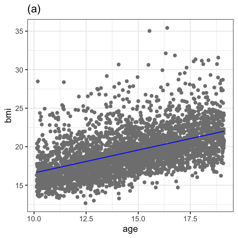
Figure 1.2 (b)
resid_qqplot(m1, value=10)+
        ggtitle("(b)")+
        theme_bw()+
        theme(legend.position = "none")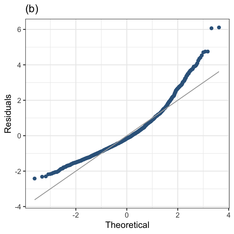
Figure 1.2 (c)
moment_bucket(m1) +
   theme_bw() +
   ggtitle("(c)") +
   theme(legend.position = "none")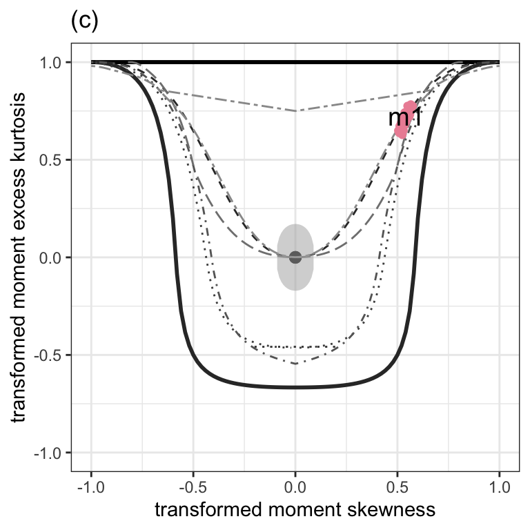
Figure 1.2 (d)
We have used the gamlss.ggplots function y_hist():
y_hist(m1$residuals, title="(d)") +
   xlab("residuals") +
theme_bw() 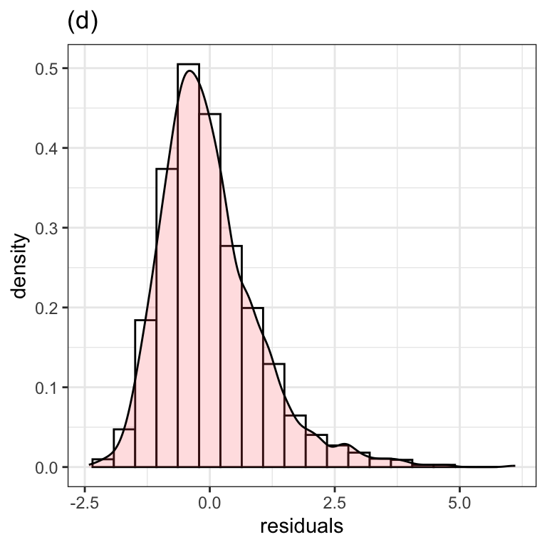
Alternatively the plot can be created using the native ggplot2 functions:
resid <- data.frame(residuals=m1$residuals)
ggplot(resid, aes(x=residuals)) +
  geom_histogram(aes(y=..density..), color="black", fill="white", bins=20) +
  geom_density(fill="pink", alpha=0.5) +
theme_bw() 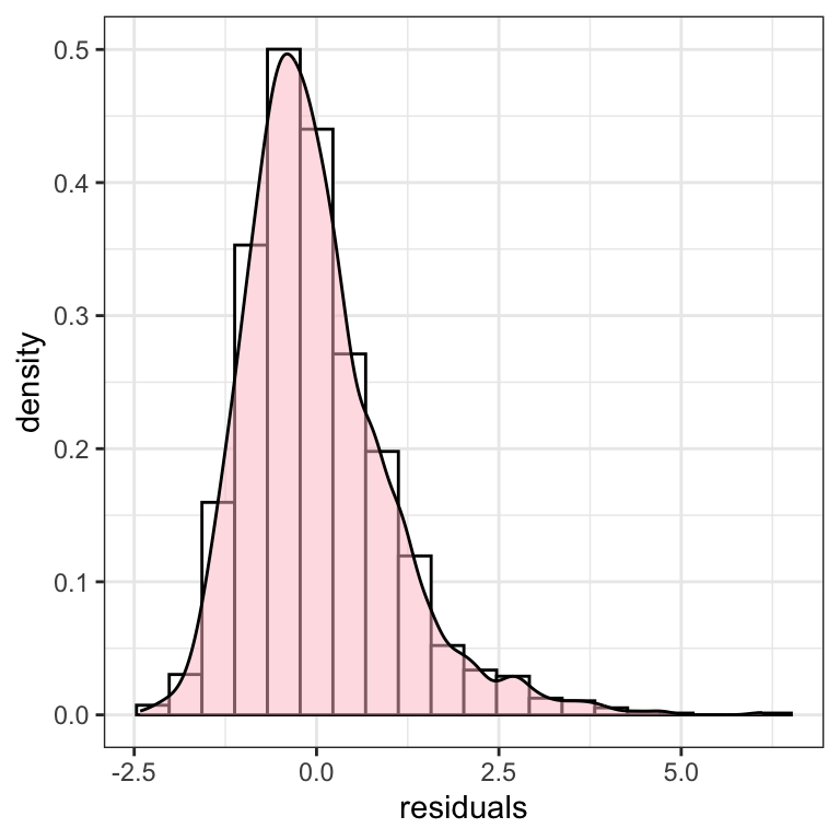
Fitting the three GAM models:
##########################################################################
# GAM models
# a GAMLSS  normal equivalent to GAM gaussian
 N <- gamlss(bmi~pb(age^(1/3)),
                 data=dbbmi, family=NO)
GAMLSS-RS iteration 1: Global Deviance = 31269.41
GAMLSS-RS iteration 2: Global Deviance = 31269.41 G <- gamlss(bmi~pb(age^(1/3)), data=dbbmi, family=GA)GAMLSS-RS iteration 1: Global Deviance = 30277.45
GAMLSS-RS iteration 2: Global Deviance = 30277.45 I <- gamlss(bmi~pb(age^(1/3)), data=dbbmi, family=IG)GAMLSS-RS iteration 1: Global Deviance = 29981.95
GAMLSS-RS iteration 2: Global Deviance = 29981.95 AIC( N, G, I) df AIC
I 12.68192 30007.31
G 12.60343 30302.66
N 12.37615 31294.16Figure 1.3 (a)
da4 <- data.frame(dbbmi, fv=fitted(I))
ggplot(data=da4, aes(x=age,  y=bmi))+
   geom_point(col="darkblue", pch=20)+
   geom_line(aes(x=age, fv), col="red", size=1.5)+
   ggtitle("(a)")+
theme_bw() 
Figure 1.3 (b)
model_qqplot(N, G, I)+
   ggtitle("(b)")+
   theme_bw()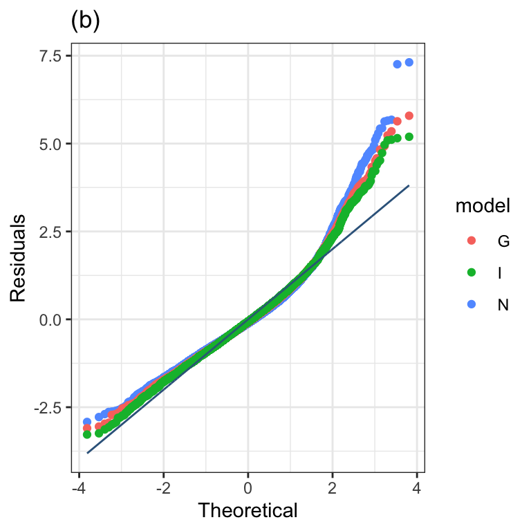
Figure 1.3 (c)
moment_bucket(N, G, I,  cex_text=7) +
   ggtitle("(c)") +
   theme_bw() +
   theme(plot.caption = element_text(hjust=0.5, size=rel(2))) +
theme(legend.position = "none") 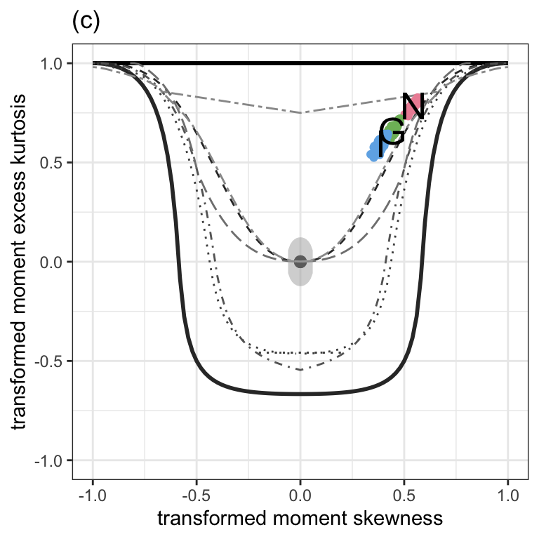
Figure 1.3 (d)
fitted_centiles(I, cent=c(97,90,75,50,25,10,3), title="(d) centiles curves") +
   theme_bw()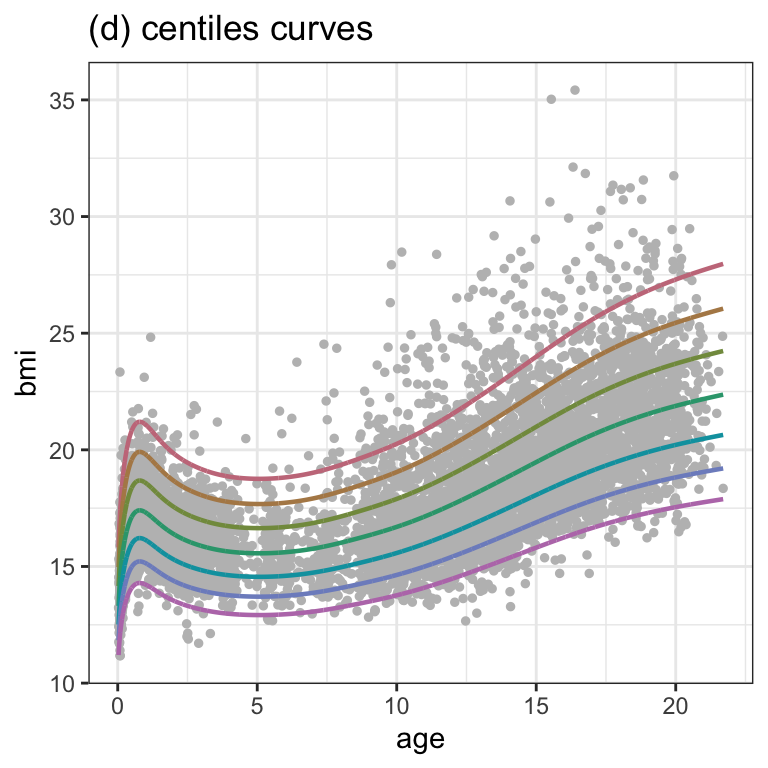
Fitting the distribution
 m2 <- gamlss(bmi~pb(age^(1/3)), sigma.fo=~pb(age^(1/3)), nu.fo=~pb(age^(1/3)),
             tau.fo=~pb(age^(1/3)),
             data=dbbmi, family=BCT)
GAMLSS-RS iteration 1: Global Deviance = 29175.74
GAMLSS-RS iteration 2: Global Deviance = 29148.08
GAMLSS-RS iteration 3: Global Deviance = 29146.78
GAMLSS-RS iteration 4: Global Deviance = 29146.58
GAMLSS-RS iteration 5: Global Deviance = 29146.53
GAMLSS-RS iteration 6: Global Deviance = 29146.51
GAMLSS-RS iteration 7: Global Deviance = 29146.51
GAMLSS-RS iteration 8: Global Deviance = 29146.51
GAMLSS-RS iteration 9: Global Deviance = 29146.51
GAMLSS-RS iteration 10: Global Deviance = 29146.51 Figure 1.5 (a)
da5 <- data.frame(dbbmi, fv=fitted(m2))
 ggplot(data=da5, aes(x=age, bmi)) +
    geom_point(col="darkblue", pch=20) +
    geom_line(aes(x=age, fv), col="red", size=1.5) +
    ggtitle("(a)") +
    theme_bw()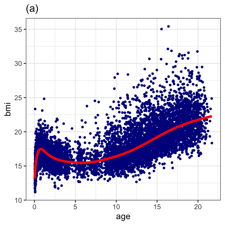
Figure 1.5 (b)
resid_qqplot(m2, value=6) +
    ggtitle("(b)") +
    theme_bw()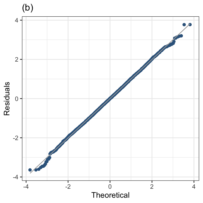
Figure 1.5 (c)
moment_bucket(m2, cex_text=6) +
    ggtitle("(c)") +
    theme_bw() +
    theme(plot.caption = element_text(hjust=0.5, size=rel(1.2))) +
theme(legend.position = "none") 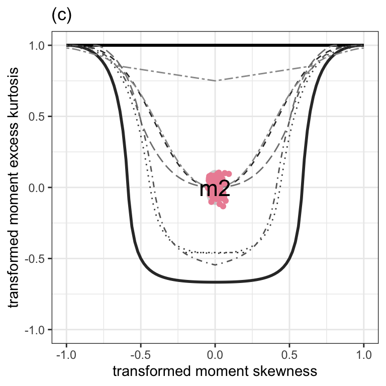
Figure 1.5 (d)
fitted_centiles(m2,  cent=c(97,90,75,50,25,10,3),  title="(d) centiles curves") +
    theme_bw()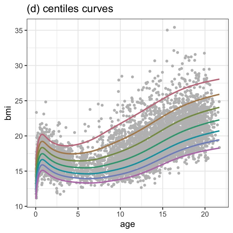
Figure 1.6 (a)
fitQR isn’t in the package
library(gamlss.foreach)
library(ggplot2)
#################################################################
# testing not in the book
q1 <- fitQR(bmi~age, data=db_bmi_10 , quantile=c(0.97,0.90,0.75,0.50, 0.25, 0.10, 0.03), c.crit=0.01)
dbbmi_e <- data.frame(db_bmi_10, fv1=fitted(q1[[1]]),
                                 fv2=fitted(q1[[2]]),
                                 fv3=fitted(q1[[3]]),
                                 fv4=fitted(q1[[4]]),
                                 fv5=fitted(q1[[5]]),
                                 fv6=fitted(q1[[6]]),
                                 fv7=fitted(q1[[7]]))
ggplot(data=dbbmi_e, aes(x=age, y=bmi))+geom_point(, col="gray") +
   geom_line(aes(x=age, y=fv1)) +
   geom_line(aes(x=age, y=fv2)) +
   geom_line(aes(x=age, y=fv3)) +
   geom_line(aes(x=age, y=fv4)) +
   geom_line(aes(x=age, y=fv5)) +
   geom_line(aes(x=age, y=fv6)) +
   geom_line(aes(x=age, y=fv7)) +
   ggtitle("(a) 10 < age < 20") +
   theme_bw()
Figure 1.6 (b)
registerDoParallel(cores = 8)
q3 <- fitQR(bmi~pb(age^(1/3)), data=dbbmi,
            quantile=c(0.97,0.90,0.75,0.50, 0.25, 0.10, 0.03), c.crit=0.01)

dbbmi_ee <- data.frame(dbbmi,
                      fv1=fitted(q3[[1]]),
                      fv2=fitted(q3[[2]]),
                      fv3=fitted(q3[[3]]),
                      fv4=fitted(q3[[4]]),
                      fv5=fitted(q3[[5]]),
                      fv6=fitted(q3[[6]]),
                      fv7=fitted(q3[[7]]))


gg <- fitted_centiles(m2,  cent=c(97,90,75,50,25,10,3), title="(b) all ages") +
  theme_bw()

gg+
   geom_line(data=dbbmi_ee, aes(x=age, y=fv1)) +
   geom_line(data=dbbmi_ee, aes(x=age, y=fv2)) +
   geom_line(data=dbbmi_ee, aes(x=age, y=fv3)) +
   geom_line(data=dbbmi_ee, aes(x=age, y=fv4)) +
   geom_line(data=dbbmi_ee, aes(x=age, y=fv5)) +
   geom_line(data=dbbmi_ee, aes(x=age, y=fv6)) +
   geom_line(data=dbbmi_ee, aes(x=age, y=fv7)) +
   theme_bw()