library(gamlss)
library(gamlss.ggplots)
library(ggplot2)9: Speech intelligibility testing
The dataset speech is in the gamlss.data package.
data(speech) Figure 9.1: Histogram of proportion of words correctly recognised
ggplot(speech, aes(x=y)) +
  geom_histogram(binwidth = 0.04, colour="darkblue", fill="lightblue") +
  xlab("Proportion correct") +
  ylab("Frequency") +
  theme_bw(base_size=14)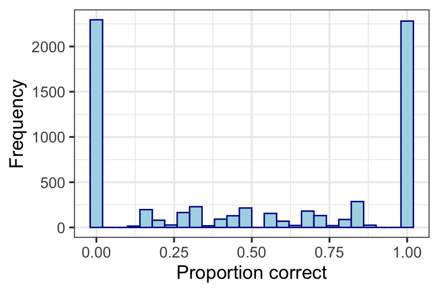
Section 9.2.1: Choice of response distribution
Use the gamlss function chooseDist() to pick the distribution for y\(\in (0,1)\), starting with the Beta (BE) distribution:
speech.01 <- subset(speech, (y>0&y<1))
m1 <- gamlss(y~snr,
             sigma.formula =~ snr,
             nu.formula =~ snr,
             tau.formula =~ snr,
             family=BE, data=speech.01, n.cyc=100, trace=FALSE)
a <- chooseDist(m1, type="real0to1")
minimum GAIC(k= 2 ) family: SIMPLEX
minimum GAIC(k= 3.84 ) family: SIMPLEX
minimum GAIC(k= 7.67 ) family: SIMPLEX The SIMPLEX is the preferred distribution for all three criteria.
Create the zero-and-one-inflated SIMPLEX distribution:
library(gamlss.inf)
gen.Inf0to1(family="SIMPLEX", type.of.Inflation = "Zero&One")
A 0to1 inflated SIMPLEX distribution has been generated
and saved under the names:
dSIMPLEXInf0to1 pSIMPLEXInf0to1 qSIMPLEXInf0to1 rSIMPLEXInf0to1
plotSIMPLEXInf0to1 9.2.2: Variable selection
library(gtools)
library(sjmisc)
Generate all model formulae to be considered:
vars<-c('snr', 'noise_dir','noise_gender','algorithm')
indexes<-unique(apply(combinations(length(vars), length(vars), repeats=T), 1, unique))
gen.form<-function(x) paste('~',paste( vars[x],collapse=' + '))
gen.form.int<-function(x) paste( interaction.vars[x],collapse=' + ')
formulas.main <-sapply(indexes, gen.form)  ## main effects
formulas.main <- c(formulas.main, "~ 1")
indexes <- c(indexes,0)
formulas <- formulas.main

# interaction terms (only interactions with algorithm)
for(i in 1:length(formulas))
{
  m <- length(indexes[[i]])
  if(m>1)
  {
    interaction.indexes <- combinations(m,2, v=indexes[[i]])
    interaction.vars <- paste(vars[interaction.indexes[,1]], ":",vars[interaction.indexes[,2]])
    # exclude interactions without algorithm
    d <- NULL
    for(j in 1:length(interaction.vars))d <- c(d, str_contains(interaction.vars[j], "algorithm"))
    interaction.vars <- interaction.vars[d]
    if(sum(d)>0)
    {
    i.indexes<-unique(apply(combinations(length(interaction.vars), length(interaction.vars),
                                         repeats=T), 1, unique))

    interaction.terms<-sapply(i.indexes, gen.form.int)
    formulas <- c(formulas, (paste(formulas[i]," + ", interaction.terms)))
    }
  }
}

n <- length(formulas)
In Figure 9.2 we show the results for \(\kappa\in \{2, 3, 4, 5, 6, 7, 8, \log(n)\}\). Here we illustrate \(\kappa=4\):
k <- 4

# starting formulas for sigma, xi0 and xi1
sigma.form <- "~ 1"
xi0.form <- xi1.form <- "~ snr"

for(N in 1:2)   ## number of times the selection is repeated
{
mu.AIC <- NULL
for(i in 1:n)
{
    eval(parse(text=paste0("m1 <- gamlssInf0to1(y=y, mu.formula =",
                               formulas[i],
                               " + random(subject), sigma.formula =", sigma.form,
                               ", xi0.formula =",xi0.form,
                               "+ random(subject), xi1.formula =",xi1.form,
                               "+ random(subject), family=SIMPLEX, data=speech, n.cyc=100)")))
    mu.AIC <- c(mu.AIC, GAIC(m1, k=k))
}
mu.form <- formulas[which.min(mu.AIC)]

sigma.AIC <- NULL
for(i in 1:n)
{
  eval(parse(text=paste0("m1 <- gamlssInf0to1(y=y, mu.formula =",mu.form,
                         ", sigma.formula =", formulas[i],
                         ", xi0.formula =",xi0.form, ", xi1.formula =",xi1.form,
                         ",family=SIMPLEX, data=speech, n.cyc=100)")))
  sigma.AIC <- c(sigma.AIC, GAIC(m1, k=k))
}
sigma.form <- formulas[which.min(sigma.AIC)]


xi0.AIC <- NULL
for(i in 1:n)
{
 eval(parse(text=paste0("m1 <- gamlssInf0to1(y=y, mu.formula =",mu.form,
                         " + random(subject), sigma.formula =", sigma.form,
                         ", xi0.formula =",formulas[i],
                         " + random(subject), xi1.formula =",xi1.form,
                         " + random(subject),family=SIMPLEX, data=speech, n.cyc=100)")))
  xi0.AIC <- c(xi0.AIC, GAIC(m1, k=k))
}
xi0.form <- formulas[which.min(xi0.AIC)]

xi1.AIC <- NULL
for(i in 1:n)
{
    eval(parse(text=paste0("m1 <- gamlssInf0to1(y=y, mu.formula =",mu.form,
                           " + random(subject), sigma.formula =", sigma.form,
                         ", xi0.formula =",xi0.form,
                         " + random(subject), xi1.formula =",formulas[i],
                         " + random(subject),family=SIMPLEX, data=speech, n.cyc=100)")))

  xi1.AIC <- c(xi1.AIC, GAIC(m1, k=k))
}
xi1.form <- formulas[which.min(xi1.AIC)]

eval(parse(text=paste0("model <- gamlssInf0to1(y=y, mu.formula =",mu.form,
                         " + random(subject), sigma.formula =", sigma.form,
                         ", xi0.formula =",xi0.form,
                         " + random(subject), xi1.formula =",xi1.form,
                         " + random(subject),family=SIMPLEX, data=speech, n.cyc=100)")))

}  ## end N
This is the chosen model, given in Table 9.2:
summary(model)*******************************************************************
Family: "InfSIMPLEX"
Call: gamlssInf0to1(y = correct, mu.formula = ~snr + noise_gender +
random(subject), sigma.formula = ~1, xi0.formula = ~snr +
noise_gender + algorithm + snr:algorithm + random(subject),
xi1.formula = ~snr + noise_gender + algorithm + random(subject),
data = bilateral, family = SIMPLEX, n.cyc = 100)
Fitting method: RS()
-------------------------------------------------------------------
Mu link function: logit
Mu Coefficients:
Estimate Std. Error t value Pr(>|t|)
(Intercept) -0.211299 0.038645 -5.468 4.72e-08 ***
snr 0.057692 0.006882 8.383 < 2e-16 ***
noise_genderM 0.109124 0.038102 2.864 0.0042 **
---
Signif. codes: 0 '***' 0.001 '**' 0.01 '*' 0.05 '.' 0.1 ' ' 1
-------------------------------------------------------------------
Sigma link function: log
Sigma Coefficients:
Estimate Std. Error t value Pr(>|t|)
(Intercept) 0.82636 0.01925 42.93 <2e-16 ***
---
Signif. codes: 0 '***' 0.001 '**' 0.01 '*' 0.05 '.' 0.1 ' ' 1
-------------------------------------------------------------------
xi0 link function: log
xi0 Coefficients:
Estimate Std. Error t value Pr(>|t|)
(Intercept) 1.13948 0.08344 13.656 < 2e-16 ***
snr -0.29338 0.02197 -13.352 < 2e-16 ***
noise_genderM -0.31877 0.05819 -5.478 4.45e-08 ***
algorithmB -0.33815 0.10217 -3.310 0.000939 ***
algorithmC -0.38921 0.10495 -3.708 0.000210 ***
snr:algorithmB 0.12101 0.02760 4.385 1.18e-05 ***
snr:algorithmC 0.03431 0.02914 1.178 0.239037
---
Signif. codes: 0 '***' 0.001 '**' 0.01 '*' 0.05 '.' 0.1 ' ' 1
-------------------------------------------------------------------
xi1 link function: log
xi1 Coefficients:
Estimate Std. Error t value Pr(>|t|)
(Intercept) -0.87799 0.07645 -11.485 < 2e-16 ***
snr 0.22358 0.01110 20.151 < 2e-16 ***
noise_genderM 0.30756 0.05790 5.311 1.12e-07 ***
algorithmB -0.09953 0.06847 -1.454 0.146
algorithmC -0.37059 0.06889 -5.380 7.72e-08 ***
---
Signif. codes: 0 '***' 0.001 '**' 0.01 '*' 0.05 '.' 0.1 ' ' 1
-------------------------------------------------------------------
NOTE: Additive smoothing terms exist in the formulas:
i) Std. Error for smoothers are for the linear effect only.
ii) Std. Error for the linear terms may not be reliable.
-------------------------------------------------------------------
No. of observations in the fit: 6720
Degrees of Freedom for the fit: 32.65723
Residual Deg. of Freedom: 6687.343
at cycle:
Global Deviance: 12228.7
AIC: 12294.02
SBC: 12516.51
*******************************************************************Figure 9.3: Worm plot
resid_wp(model, title=NULL, value=10)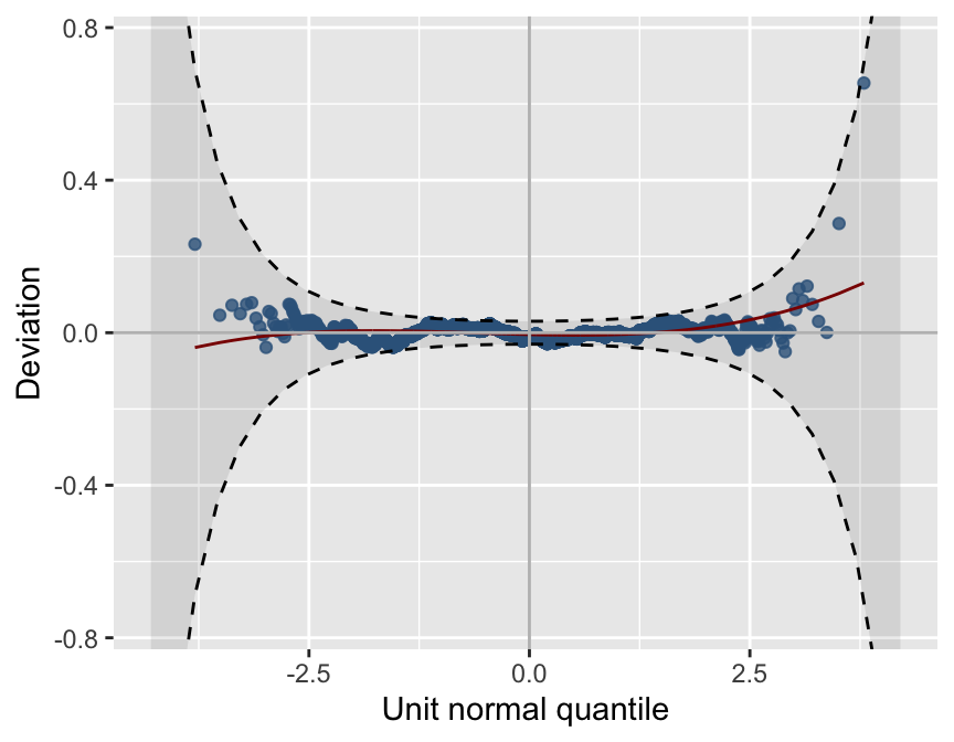
Section 9.3: Compute fitted values and bootstrap confidence intervals
Function pred.re() to compute fitted values
The generic pred() function was found not to work when the model includes random effects. The following function pred.re() does it:
pred.re <- function(mod, newdata, z=0, random=FALSE, seed=3876)
{
  ## obtains predictions for SIMPLEX01 (predict doesn't work with random effects)
  preds <- newdata
  re <- data.frame(subject=unique(preds$subject))
  m <- nrow(re)
  if(random)
  {
  set.seed(seed)
  re$mu.re <-  rnorm(m)
  re$sigma.re <-  rnorm(m)
  re$xi0.re <-  rnorm(m)
  re$xi1.re <-  rnorm(m)
  } else re$mu.re <- re$sigma.re <- re$xi0.re <- re$xi1.re <- z
  mu.re.expanded <- rep(re$mu.re, times=unclass(table(preds$subject)))
  sigma.re.expanded <- rep(re$sigma.re, times=unclass(table(preds$subject)))
  xi0.re.expanded <- rep(re$xi0.re, times=unclass(table(preds$subject)))
  xi1.re.expanded <- rep(re$xi1.re, times=unclass(table(preds$subject)))

  # leave out random effects
  mod$mu.coefficients <- na.omit(mod$mu.coefficients)
  mod$sigma.coefficients <- na.omit(mod$sigma.coefficients)
  mod$xi0.coefficients <- na.omit(mod$xi0.coefficients)
  mod$xi1.coefficients <- na.omit(mod$xi1.coefficients)

  pmu <- length(mod$mu.coefficients)
  psigma <- length(mod$sigma.coefficients)
  pxi0 <- length(mod$xi0.coefficients)
  pxi1 <- length(mod$xi1.coefficients)

  # obtain summary object, but suppress summary output
  sink(file="temp")
  a=summary(mod)
  sink()
  file.remove("temp")

  mu.se <- a[1:pmu,2]
  sigma.se <- a[(pmu+1):(pmu+psigma),2]
  xi0.se <- a[(pmu+psigma+1):(pmu+psigma+pxi0),2]
  xi1.se <- a[(pmu+psigma+pxi0+1):(pmu+psigma+pxi0+pxi1),2]

  mu.lp <- rep(mod$mu.coefficients[1], nrow(newdata))
  for(j in 2:length(mod$mu.coefficients))
  {
    var <- names(mod$mu.coefficients)[j]
    if(var!="random(subject)")
      mu.lp <- mu.lp + newdata[,which(names(newdata)==var)]*mod$mu.coefficients[j]
    else mu.lp <- mu.lp + mu.re.expanded*mu.se[j]
  }
  preds$mu <- exp(mu.lp)/(1+exp(mu.lp))

  p <- length(mod$sigma.coefficients)
  sigma.lp <- rep(mod$sigma.coefficients[1], nrow(newdata))
  if(p>1)for(j in 2:(p-1))
    sigma.lp <-
        sigma.lp +
        newdata[,which(names(newdata)==names(mod$sigma.coefficients)[j])]*mod$sigma.coefficients[j]
  preds$sigma <- exp(sigma.lp)

  xi0.lp <- rep(mod$xi0.coefficients[1], nrow(newdata))
  for(j in 2:length(mod$xi0.coefficients))
  {
    var <- names(mod$xi0.coefficients)[j]
    if(var!="random(subject)")
      xi0.lp <- xi0.lp + newdata[,which(names(newdata)==var)]*mod$xi0.coefficients[j]
    else xi0.lp <- xi0.lp + xi0.re.expanded*xi0.se[j]
  }
  preds$xi0 <- exp(xi0.lp)

  xi1.lp <- rep(mod$xi1.coefficients[1], nrow(newdata))
  for(j in 2:length(mod$xi1.coefficients))
  {
    var <- names(mod$xi1.coefficients)[j]
    if(var!="random(subject)")
      xi1.lp <- xi1.lp + newdata[,which(names(newdata)==var)]*mod$xi1.coefficients[j]
    else xi1.lp <- xi1.lp + xi1.re.expanded*xi1.se[j]
  }
  preds$xi1 <- exp(xi1.lp)

  preds$p0 <- preds$xi0/(1+preds$xi0+preds$xi1)
  preds$p1 <- preds$xi1/(1+preds$xi0+preds$xi1)
  preds$overallmean <- preds$mu*(1-preds$p0-preds$p1) + preds$p1

  return(preds)
}
Compute and plot fitted values for \(\xi_0\), \(\xi_1\) and percent overall correct
Set up the data frame newdata for prediction:
library(fastDummies)

g <- c("F","M")
a <- c("A","B","C")
s <- seq(-5,15, by=0.25)
newdata <- data.frame(expand.grid(g,a,s))
names(newdata) <- c("noise_gender", "algorithm","snr")
newdata$noise_dir <- "F"
newdata$correct <- 0
newdata$subject <- "B2"
newdata <- dummy_cols(newdata, select_columns=c("noise_gender", "algorithm","noise_dir"),
                      remove_first_dummy = TRUE)
names(newdata)[7:10] <- c("noise_genderM", "algorithmB" ,   "algorithmC" ,   "noise_dirS")
newdata$'snr:algorithmB' <- newdata$snr*newdata$algorithmB
newdata$'snr:algorithmC' <- newdata$snr*newdata$algorithmC
newdata$'noise_dirS:algorithmB' <- newdata$noise_dirS*newdata$algorithmB
newdata$'noise_dirS:algorithmC' <- newdata$noise_dirS*newdata$algorithmC
newdata$'noise_genderM:algorithmB' <- newdata$noise_genderM*newdata$algorithmB
newdata$'noise_genderM:algorithmC' <- newdata$noise_genderM*newdata$algorithmC
Compute predictions:
preds <- pred.re(model, newdata, z=0)Plot predictions
- Fitted proportion zero correct: \(\hat\xi_0\)
ggplot(preds, aes(x=snr, y=p0, colour=algorithm)) +
  geom_line(size=1.0) +
  facet_grid(.~noise_gender)+
  ylab("Fitted proportion zero correct") + xlab("SNR") +
  scale_y_continuous(labels=scales::percent) +
  theme_bw()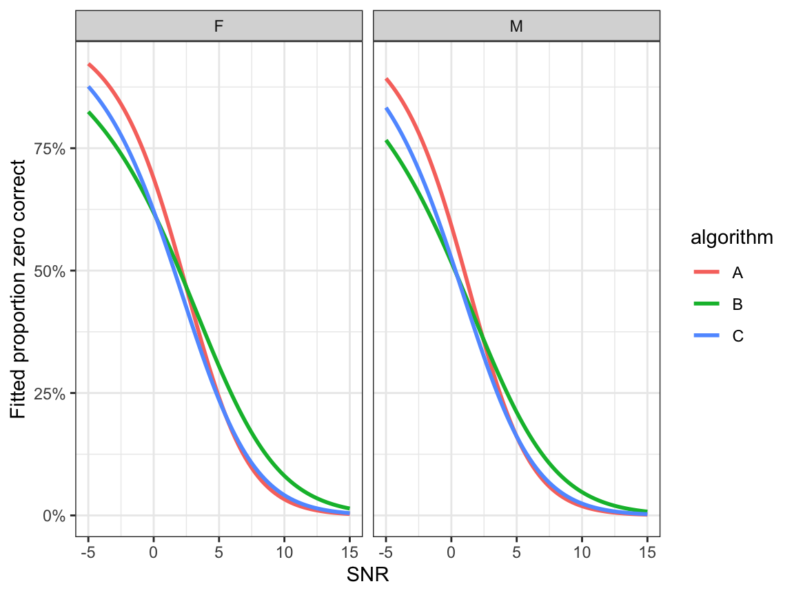
- Fitted proportion all correct: \(\hat\xi_1\)
ggplot(preds, aes(x=snr, y=p1, colour=algorithm)) +
  geom_line(size=1.0) +
  facet_grid(.~noise_gender)+
  ylab("Fitted proportion all correct") + xlab("SNR") +
  scale_y_continuous(labels=scales::percent) +
  theme_bw()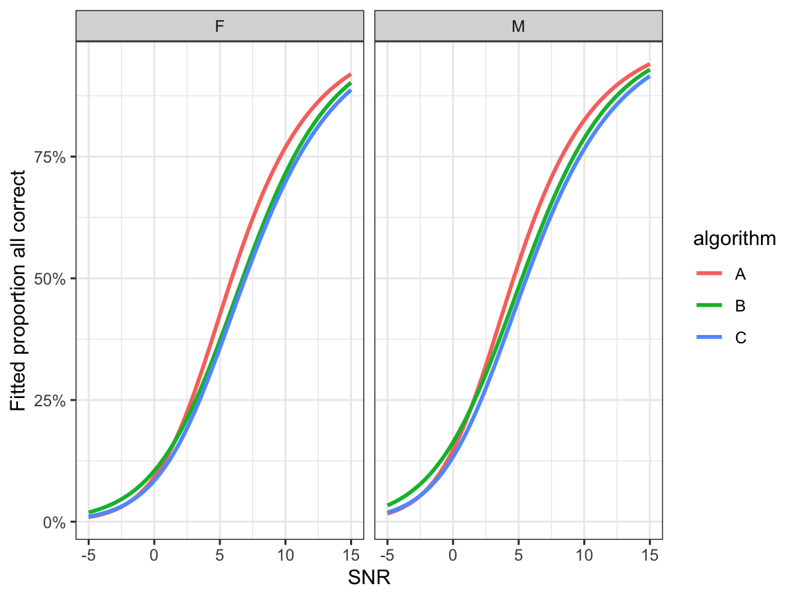
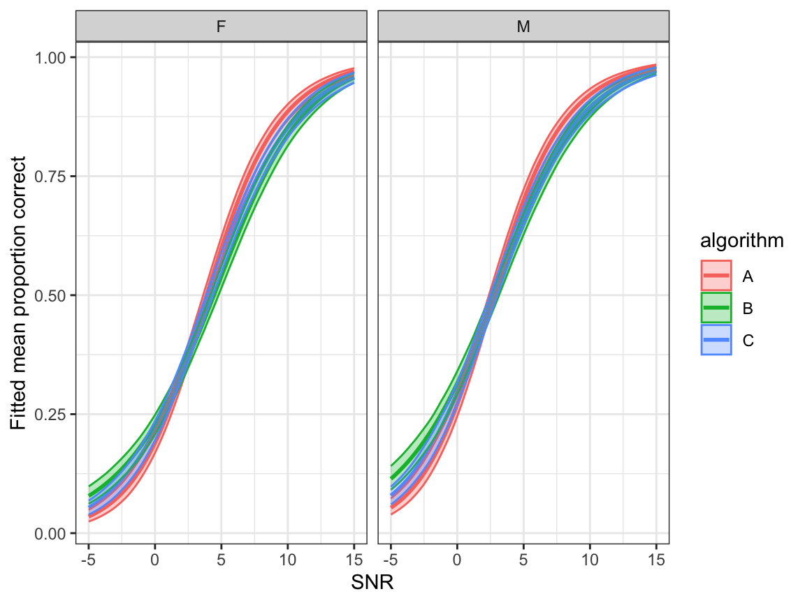
- Fitted overall mean correct (equation (9.4)) \[ \hat{\mathbb{E}}(y)=\frac{\hat{\mu}+\hat{\xi}_1}{1+\hat{\xi}_0+\hat{\xi}_1} \]
ggplot(preds, aes(x=snr, y=overallmean, colour=algorithm)) +
  geom_line(size=1.0) +
  facet_grid(.~noise_gender)+
  ylab("Fitted overall mean") + xlab("SNR") +
  scale_y_continuous(labels=scales::percent) +
  theme_bw()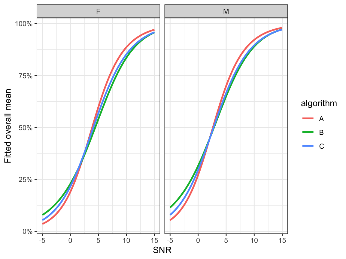
Figure 9.4
Compute bootstrap confidence intervals
# original sample
original <- speech[,c("noise_gender","algorithm" , "snr" , "noise_dir" , "y" ,"subject" )]
original <-
  dummy_cols(original, select_columns=c("noise_gender", "algorithm", "noise_dir"),
             remove_first_dummy = TRUE)
names(original)[7:10] <- c("noise_genderM", "algorithmB", "algorithmC", "noise_dirS")
original$'snr:algorithmB' <- original$snr*original$algorithmB
original$'snr:algorithmC' <- original$snr*original$algorithmC
original$'noise_dirS:algorithmB' <- original$noise_dirS*original$algorithmB
original$'noise_dirS:algorithmC' <- original$noise_dirS*original$algorithmC
original$'noise_genderM:algorithmB' <- original$noise_genderM*original$algorithmB
original$'noise_genderM:algorithmC' <- original$noise_genderM*original$algorithmC

# this takes a while!
B <- 500
n <- nrow(original)
bootsam <- original
bootmeans <- bootp0 <- bootp1 <- NULL
set.seed(9371)
preds <- pred.re(model, original, random=TRUE)

for(b in 1:B)
{
  cat(b,"\n")
  yboot <- rSIMPLEXInf0to1(n, mu=preds$mu, sigma=preds$sigma, xi0=preds$xi0, xi1=preds$xi1)
  bootsam$correct <- yboot
  eval(parse(text=paste0("mboot <- gamlssInf0to1(y=correct, mu.formula =",
                         paste("~ ",paste(names(model$mu.coefficients)[-1], collapse=" + ")),
                         ", sigma.formula = ~1, xi0.formula =",
                         paste("~ ",paste(names(model$xi0.coefficients)[-1], collapse=" + ")),
                         ", xi1.formula =",
                         paste("~ ",paste(names(model$xi1.coefficients)[-1], collapse=" + ")),
                         ", family=SIMPLEX, data=bootsam, n.cyc=100)")))
bootmeans <- cbind(bootmeans, pred.re(mboot, newdata)$overallmean )
bootp0 <- cbind(bootp0, pred.re(mboot, newdata)$p0 )
bootp1 <- cbind(bootp1, pred.re(mboot, newdata)$p1 )

}

bootdata <- pred.re(model, newdata)
bootdata <-
  cbind(bootdata,
    lower=apply(bootmeans, 1, quantile, probs=0.025),
    upper=apply(bootmeans, 1, quantile, probs=0.975),
    p0lower=apply(bootp0, 1, quantile, probs=0.025),
    p0upper=apply(bootp0, 1, quantile, probs=0.975),
    p1lower=apply(bootp1, 1, quantile, probs=0.025),
    p1upper=apply(bootp1, 1, quantile, probs=0.975))
Plot predictions with bootstrap confidence intervals
- Fitted proportion zero correct: \(\hat\xi_0\)
ggplot(bootdata, aes(x=snr,y=p0,colour=algorithm, fill=algorithm)) +
  geom_line(linewidth=1.0) +
  geom_ribbon(aes(ymin = p0lower, ymax = p0upper), alpha = 0.3)+
  facet_grid(.~noise_gender)+
  ylab("Fitted proportion zero correct") + xlab("SNR") +
  scale_y_continuous()+
  theme_bw()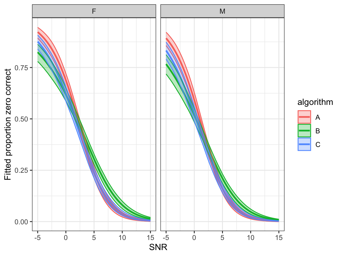
- Fitted proportion all correct: \(\hat\xi_1\)
ggplot(bootdata, aes(x=snr,y=p1,colour=algorithm, fill=algorithm)) +
  geom_line(linewidth=1.0) +
  geom_ribbon(aes(ymin = p1lower, ymax = p1upper), alpha = 0.3)+
  facet_grid(.~noise_gender)+
  ylab("Fitted proportion all correct") + xlab("SNR") +
  scale_y_continuous()+
  theme_bw()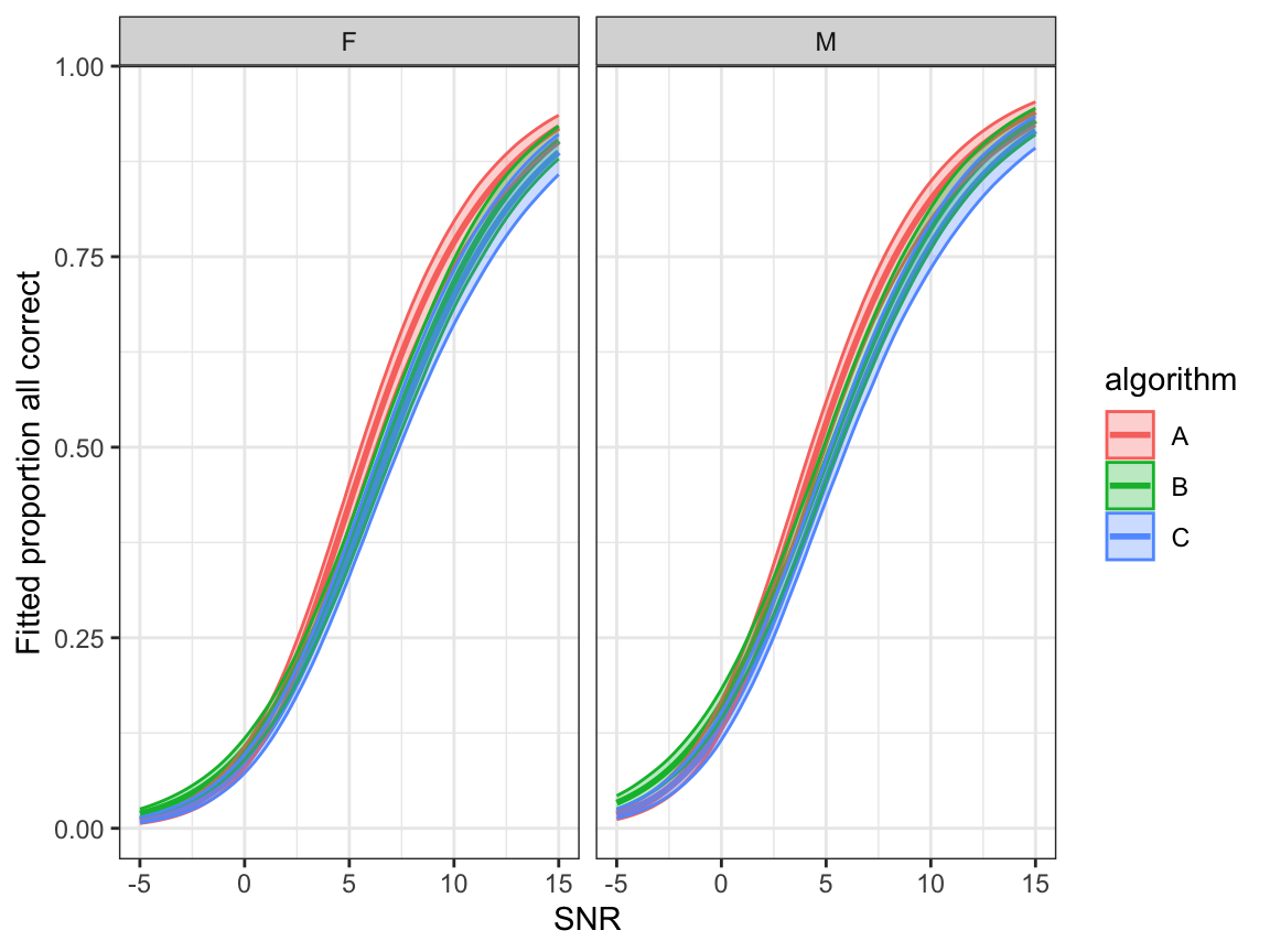
- Fitted overall mean correct (equation (9.4)) \[ \hat{\mathbb{E}}(y)=\frac{\hat{\mu}+\hat{\xi}_1}{1+\hat{\xi}_0+\hat{\xi}_1} \]
ggplot(bootdata, aes(x=snr,y=overallmean,colour=algorithm, fill=algorithm)) +
  geom_line(linewidth=1.0) +
  geom_ribbon(aes(ymin = lower, ymax = upper), alpha = 0.3)+
  facet_grid(.~noise_gender)+
  ylab("Fitted mean proportion correct") + xlab("SNR") +
  scale_y_continuous()+
  theme_bw()