library(gamboostLSS)
library(mboost)
library(mgcv)
library(gamlss)
library(moments)7: Statistical Boosting for GAMLSS
Illustrating the behaviour of statistical boosting
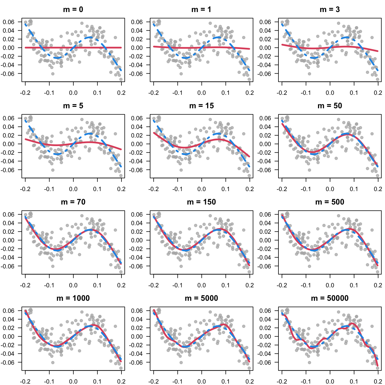
Figure 7.6
Figure 7.6 illustrates the fitting of non-linear effects via statistical boosting by highlighting how the number of iterations influences the roughness or smoothness of the fit.
The code first simulates an artificial data example, afterwards a univariate GAM is fitted with different stopping iterations.
###########################################################
## Simulate data
###########################################################

## uniformly distributed covariate
x <- runif(150, -0.2, 0.2)

## outcome following a pre-defined curve + noise
y <- -(.4 - 0.95* exp(-50*x^2))*x + 0.02 *rnorm(150)

y <- y[order(x)] ## order obs by size of x
x <- x[order(x)] ## just for easier plotting

plot(x, y, pch = 19)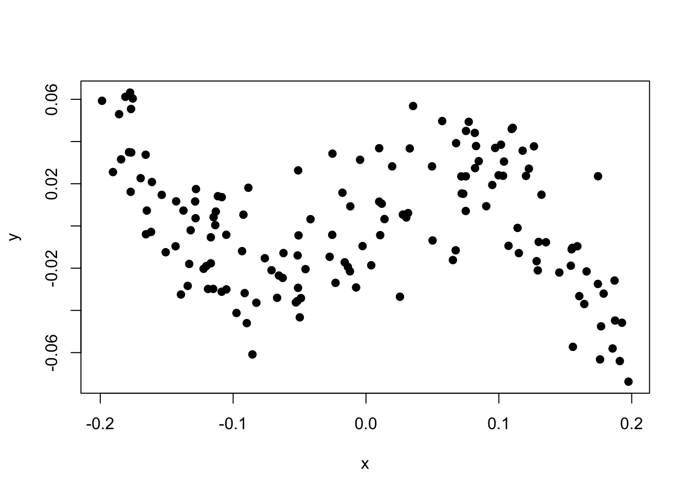
###########################################################
## Plotting
###########################################################
par(
  mfrow = c(4, 3),
  mar = c(2, 3, 2.5, 0.5),
  cex.main = 1.3
)
plot(
  x,
  y,
  las = 1,
  main = "m = 0",
  pch = 19,
  xlab = "",
  ylab = "",
  col = rgb(0.7, 0.7, 0.7, 0.75)
) ## observations
## now carry out one boosting iteration
gam1 <- gamboost(y ~ x, control = boost_control(mstop = 0))
lines(x , fitted(gam1), lwd = 3, col = 2)
## add true function
curve(
  -(.4 - 0.95 * exp(-50 * x ^ 2)) * x,
  add = TRUE,
  from = -.2,
  to = .2,
  lty = 4,
  lwd = 3,
  col = 4
)

## for a sequence of iterations
it_values <- c(1, 3, 5, 15,  50, 70, 150, 500,
               1000,  5000, 50000)
for (j in it_values) {
  plot(
    x,
    y,
    las = 1,
    main = paste("m =", j),
    pch = 19,
    xlab = "",
    ylab = "",
    col = rgb(0.7, 0.7, 0.7, 0.75)
  ) ## observations
  lines(x , fitted(gam1[j]), lwd = 3, col = 2)
  curve(
    -(.4 - 0.95 * exp(-50 * x ^ 2)) * x,
    add = TRUE,
    from = -.2,
    to = .2,
    lty = 4,
    lwd = 3,
    col = 4
  )
}
Determine the optimal stopping iterations mstop
set.seed(2305)

## set initial value
mstop(gam1) <- 500

## 25-fold bootstrap
cvr <- cvrisk(gam1)

## results
plot(cvr)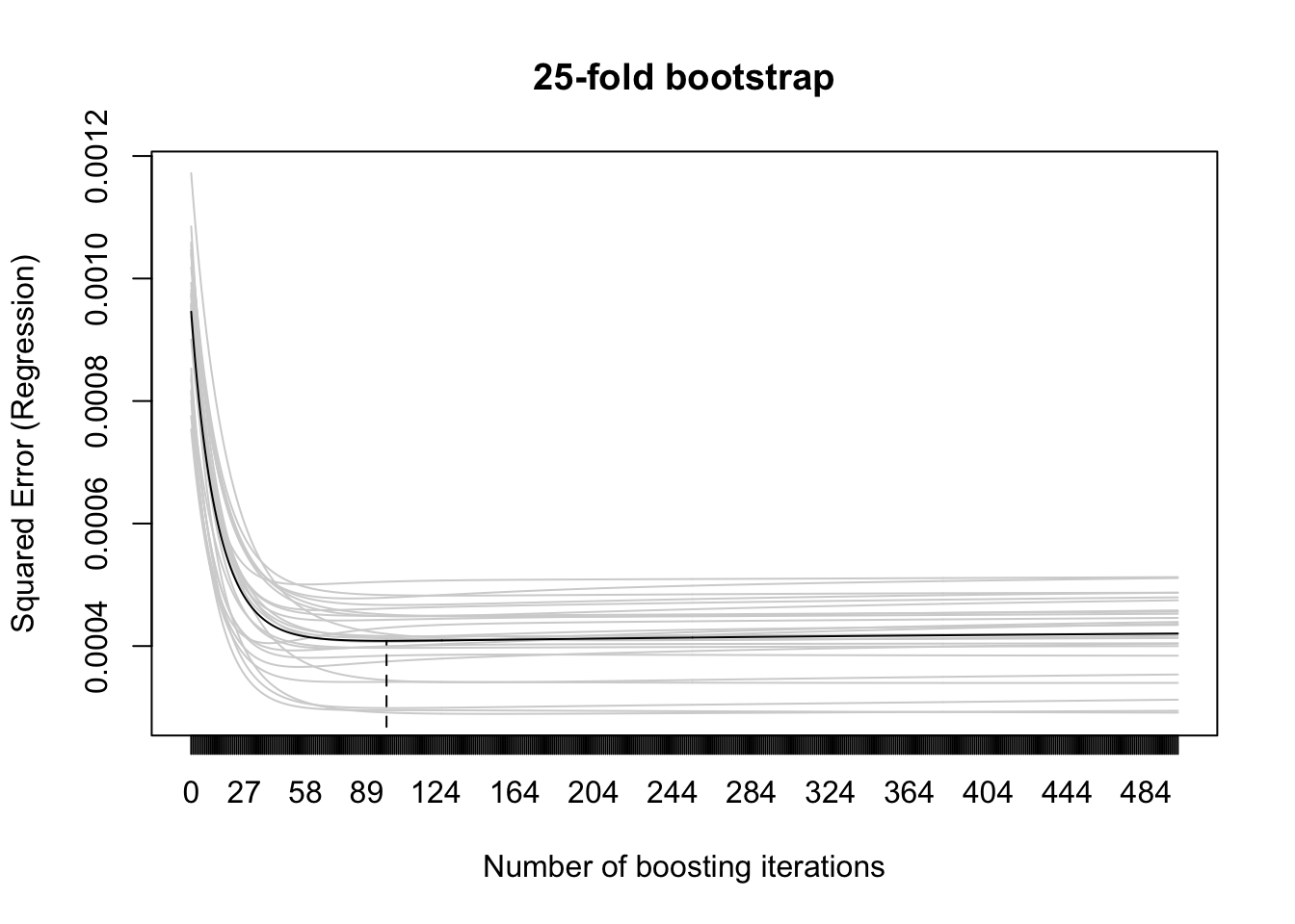
## resulting optimal mstop
mstop(cvr)
[1] 99Birthweight prediction
load(file="data/Ultra.RData")
ultra$logAC <- log(ultra$AC)
ultra$logbw <- log(ultra$birthweight)
ultra$int <- rep(1, nrow(ultra))
Table 7.1
Table 7.1. compares the results of boosting prediction models with classical inference schemes. Four different models are estimated via both approaches in a 10-fold cross-validation. The performance is compared via MAPE, MPE and RE (sd of percentage error).
The fitting is embedded in a function ‘AMP’ that is applied in parallel (if a parallel computing environment is available) on each of the folds.
AMP <- function(id) {
  set.seed(2305)
  cvd <- cv(type = "kfold", weights = rep(1, nrow(ultra)))

  dat.train <- ultra[cvd[, id] == 1, ]
  dat.test <- ultra[cvd[, id] == 0, ]

  set.seed(id)
  # classical linear model
  glm1 <-
    glmboost(logbw ~ logAC + HC + FL + BPD + Daysbeforedelivery + parity + age,
             data = dat.train)
  cvr <-
    cvrisk(
      folds = cv(weights = model.weights(glm1), type = "bootstrap"),
      glm1,
      grid = 1:1000
    )
  mstop(glm1) <- mstop(cvr)


  pred_glm1 <- exp(predict(glm1, newdata = dat.test))
  pe_glm1 <-
    100 * (dat.test$babyweight - pred_glm1) / dat.test$babyweight
  aep_glm1 <- abs(pe_glm1)
  length_glm1 <- length(coef(glm1))


  lm1 <-
    lm(logbw ~ logAC + HC + FL + BPD + Daysbeforedelivery + parity + age ,
       data = dat.train)


  pred_lm1 <- exp(predict(lm1, newdata = dat.test))
  pe_lm1 <- 100 * (dat.test$babyweight - pred_lm1) / dat.test$babyweight
  aep_lm1 <- abs(pe_lm1)
  length_lm1 <- length(coef(lm1))

  set.seed(id)
  # linear model with pairwise interactions
  glm2 <-
    glmboost(
      logbw ~ logAC +  HC + FL + BPD + Daysbeforedelivery + parity + age +
        logAC:HC + logAC:FL + logAC:BPD + logAC:Daysbeforedelivery + logAC:parity + logAC:age +
        HC:FL + HC:BPD + HC:Daysbeforedelivery + HC:parity + HC:age +
        FL:BPD + FL:Daysbeforedelivery + FL:parity + FL:age +
        BPD:Daysbeforedelivery + BPD:parity + BPD:age +
        Daysbeforedelivery:parity + Daysbeforedelivery:age +
        parity:age,
      data = dat.train
    )
  cvr <-
    cvrisk(
      folds = cv(weights = model.weights(glm2), type = "bootstrap"),
      glm2,
      grid = 1:5000
    )
  mstop(glm2) <- mstop(cvr)


  pred_glm2 <- exp(predict(glm2, newdata = dat.test))
  pe_glm2 <-
    100 * (dat.test$babyweight - pred_glm2) / dat.test$babyweight
  aep_glm2 <- abs(pe_glm2)
  length_glm2 <- length(coef(glm2))

  lm2 <-
    lm(
      logbw ~ logAC +  HC + FL + BPD + Daysbeforedelivery + parity + age +
        logAC:HC + logAC:FL + logAC:BPD + logAC:Daysbeforedelivery + logAC:parity + logAC:age +
        HC:FL + HC:BPD + HC:Daysbeforedelivery + HC:parity + HC:age +
        FL:BPD + FL:Daysbeforedelivery + FL:parity + FL:age +
        BPD:Daysbeforedelivery + BPD:parity + BPD:age +
        Daysbeforedelivery:parity + Daysbeforedelivery:age +
        parity:age ,
      data = dat.train
    )


  pred_lm2 <- exp(predict(lm2, newdata = dat.test))
  pe_lm2 <- 100 * (dat.test$babyweight - pred_lm2) / dat.test$babyweight
  aep_lm2 <- abs(pe_lm2)
  length_lm2 <- length(coef(lm2))


  set.seed(id)
  # linear model with all interactions
  glm3 <-
    glmboost(logbw ~ logAC *  HC * FL * BPD * Daysbeforedelivery * parity * age ,
             data = dat.train)
  cvr <-
    cvrisk(
      folds = cv(weights = model.weights(glm3), type = "bootstrap"),
      glm3,
      grid = 1:5000
    )
  mstop(glm3) <- mstop(cvr)


  pred_glm3 <- exp(predict(glm3, newdata = dat.test))
  pe_glm3 <-
    100 * (dat.test$babyweight - pred_glm3) / dat.test$babyweight
  aep_glm3 <- abs(pe_glm3)
  length_glm3 <- length(coef(glm3))

  lm3 <-
    lm(logbw ~ logAC *  HC * FL * BPD * Daysbeforedelivery * parity * age ,
       data = dat.train)


  pred_lm3 <- exp(predict(lm3, newdata = dat.test))
  pe_lm3 <- 100 * (dat.test$babyweight - pred_lm3) / dat.test$babyweight
  aep_lm3 <- abs(pe_lm3)
  length_lm3 <- length(coef(lm3))

  set.seed(id)
  # non-linear model
  gam1 <-
    gamboost(
      logbw ~ bols(int, intercept = FALSE) +  logAC  +  HC + FL + BPD  + Daysbeforedelivery
      + bols(parity)  + age,
      data = dat.train
    )
  cvr <-
    cvrisk(
      folds = cv(weights = model.weights(gam1), type = "bootstrap"),
      gam1,
      grid = 1:1000
    )
  mstop(gam1) <- mstop(cvr)


  pred_gam1 <- exp(predict(gam1, newdata = dat.test))
  pe_gam1 <-
    100 * (dat.test$babyweight - pred_gam1) / dat.test$babyweight
  aep_gam1 <- abs(pe_gam1)
  length_gam1 <- length(coef(gam1))


  mgcv1 <-
    gam(logbw ~ s(logAC) +  s(HC) +  s(FL) + s(BPD) + s(Daysbeforedelivery) + parity + s(age),
        data = dat.train)


  pred_mgcv <- exp(predict(mgcv1, newdata = dat.test))
  pe_mgcv <-
    100 * (dat.test$babyweight - pred_mgcv) / dat.test$babyweight
  aep_mgcv <- abs(pe_mgcv)
  length_mgcv <- length(coef(mgcv1))

  return(
    list(
      aep_glm1,
      aep_lm1,
      aep_glm2,
      aep_lm2,
      aep_glm3,
      aep_lm3,
      aep_gam1,
      aep_mgcv,
      pe_glm1,
      pe_lm1,
      pe_glm2,
      pe_lm2,
      pe_glm3,
      pe_lm3,
      pe_gam1,
      pe_mgcv,
      pred_glm1,
      pred_lm1,
      pred_glm2,
      pred_lm2,
      pred_glm3,
      pred_lm3,
      pred_gam1,
      pred_mgcv,
      dat.test$babyweight,
      length_glm1,
      length_lm1,
      length_glm2,
      length_lm2,
      length_glm3,
      length_lm3,
      length_gam1,
      length_mgcv
    )
  )
}
This is now executed 10 times on the different fold, the results are stored in a list.
library(parallel)

id <- 1:10
ERG <- mclapply(id, FUN = AMP, mc.cores = 10, mc.preschedule = FALSE)
Now the results are extracted and the Table is built.
aep_glm1 <- unlist(lapply(ERG, FUN= function(x) x[[1]]))
aep_lm1 <-  unlist(lapply(ERG, function(x)  x[[2]]))
aep_glm2 <- unlist(lapply(ERG, function(x) x[[3]]))
aep_lm2 <- unlist( lapply(ERG, function(x)  x[[4]]))
aep_glm3 <- unlist(lapply(ERG, function(x) x[[5]]))
aep_lm3 <- unlist(lapply(ERG, function(x)  x[[6]]))
aep_gam1 <- unlist(lapply(ERG, function(x) x[[7]]))
aep_mgcv <- unlist(lapply(ERG, function(x) x[[8]]))

pe_glm1 <- unlist(lapply(ERG, function(x) x[[9]]))
pe_lm1 <-  unlist(lapply(ERG, function(x) x[[10]]))
pe_glm2 <- unlist(lapply(ERG, function(x) x[[11]]))
pe_lm2 <- unlist( lapply(ERG, function(x) x[[12]]))
pe_glm3 <- unlist(lapply(ERG, function(x) x[[13]]))
pe_lm3 <- unlist(lapply(ERG, function(x)  x[[14]]))
pe_gam1 <- unlist(lapply(ERG, function(x) x[[15]]))
pe_mgcv <- unlist(lapply(ERG, function(x) x[[16]]))

pred_glm1 <- unlist(lapply(ERG, function(x) x[[17]]))
pred_lm1 <-  unlist(lapply(ERG, function(x) x[[18]]))
pred_glm2 <- unlist(lapply(ERG, function(x) x[[19]]))
pred_lm2 <- unlist( lapply(ERG, function(x) x[[20]]))
pred_glm3 <- unlist(lapply(ERG, function(x) x[[21]]))
pred_lm3 <- unlist(lapply(ERG, function(x)  x[[22]]))
pred_gam1 <- unlist(lapply(ERG, function(x) x[[23]]))
pred_mgcv <- unlist(lapply(ERG, function(x) x[[24]]))

bw <- unlist(sapply(ERG, function(x) x[[25]]))


length_glm1 <- unlist(lapply(ERG, function(x) x[[26]]))
length_lm1 <-  unlist(lapply(ERG, function(x) x[[27]]))
length_glm2 <- unlist(lapply(ERG, function(x) x[[28]]))
length_lm2 <- unlist( lapply(ERG, function(x) x[[29]]))
length_glm3 <- unlist(lapply(ERG, function(x) x[[30]]))
length_lm3 <- unlist(lapply(ERG, function(x)  x[[31]]))
length_gam1 <- unlist(lapply(ERG, function(x) x[[32]]))
length_mgcv <- unlist(lapply(ERG, function(x) x[[33]]))


tab <-
  cbind(
    median(aep_lm1),
    median(aep_glm1),
    median(aep_lm2),
    median(aep_glm2),
    median(aep_lm3),
    median(aep_glm3),
    median(aep_mgcv),
    median(aep_gam1)
  )
tab <- rbind(tab,
             c(
               mean(pe_lm1),
               mean(pe_glm1),
               mean(pe_lm2),
               mean(pe_glm2),
               mean(pe_lm3),
               mean(pe_glm3),
               mean(pe_mgcv),
               mean(pe_gam1)
             ))
tab <- rbind(tab,
             c(
               sd(pe_lm1),
               sd(pe_glm1),
               sd(pe_lm2),
               sd(pe_glm2),
               sd(pe_lm3),
               sd(pe_glm3),
               sd(pe_mgcv),
               sd(pe_gam1)
             ))
tab <- rbind(tab,
             c(
               mean(length_lm1),
               mean(length_glm1),
               mean(length_lm2),
               mean(length_glm2),
               mean(length_lm3),
               mean(length_glm3),
               mean(length_mgcv),
               mean(length_gam1)
             ) - 1)


colnames(tab) <-
  c(
    "model1",
    "model1 boosting",
    "model2",
    "model2 boosting",
    "model3",
    "model3 boosting",
    "model4",
    "model4 boosting"
  )
rownames(tab) <-
  c(
    "median absolute percentage error",
    "mean percentage error",
    "sd percentage error" ,
    "length"
  )
round(t(tab), 2)
median absolute percentage error mean percentage error
model1 5.92 -0.45
model1 boosting 5.90 -0.45
model2 5.63 -0.46
model2 boosting 5.66 -0.44
model3 5.87 -1.34
model3 boosting 5.43 -0.49
model4 5.80 -0.44
model4 boosting 5.79 -0.46
sd percentage error length
model1 9.54 7.0
model1 boosting 9.55 7.0
model2 9.22 28.0
model2 boosting 9.16 17.0
model3 19.94 127.0
model3 boosting 9.31 19.4
model4 9.32 55.0
model4 boosting 9.43 6.0Table 7.2 (L2 vs L1)
Table 7.2 of the book compares the performance of L2-boosting with boosting median regression, e.g. optimizing the L1 loss. The prediction accuracy is compared via 10-fold cross-validation.
AMP <- function(id) {
  set.seed(2305)
  cvd <- cv(type = "kfold", weights = rep(1, nrow(ultra)))

  # generate train and test data
  dat.train <- ultra[cvd[, id] == 1, ]
  dat.test <- ultra[cvd[, id] == 0, ]

  set.seed(id)
  # quantile regression model
  glm1 <-
    glmboost(
      logbw ~ logAC + HC + FL + BPD
      + Daysbeforedelivery + parity + age,
      data = dat.train,
      family = QuantReg()
    )
  cvr <-
    cvrisk(
      folds = cv(weights = model.weights(glm1), type = "bootstrap"),
      glm1,
      grid = 1:5000
    )
  mstop(glm1) <- mstop(cvr)


  pred_glm1 <- exp(predict(glm1, newdata = dat.test))
  pe_glm1 <-
    100 * (dat.test$babyweight - pred_glm1) / dat.test$babyweight
  aep_glm1 <- abs(pe_glm1)
  length_glm1 <- length(coef(glm1))

  set.seed(id)
  lm1 <-
    glmboost(
      logbw ~ logAC + HC + FL + BPD
      + Daysbeforedelivery + parity + age ,
      data = dat.train,
      family = Gaussian()
    )
  cvr <-
    cvrisk(
      folds = cv(weights = model.weights(lm1), type = "bootstrap"),
      lm1,
      grid = 1:1000
    )
  mstop(lm1) <- mstop(cvr)


  set.seed(id)
  pred_lm1 <- exp(predict(lm1, newdata = dat.test))
  pe_lm1 <- 100 * (dat.test$babyweight - pred_lm1) / dat.test$babyweight
  aep_lm1 <- abs(pe_lm1)
  length_lm1 <- length(coef(lm1))

  set.seed(id)
  # linear model with pairwise interactions
  glm2 <-
    glmboost(
      logbw ~ logAC +  HC + FL + BPD +
        Daysbeforedelivery + parity + age +
        logAC:HC + logAC:FL + logAC:BPD +
        logAC:Daysbeforedelivery + logAC:parity + logAC:age +
        HC:FL + HC:BPD + HC:Daysbeforedelivery +
        HC:parity + HC:age +
        FL:BPD + FL:Daysbeforedelivery + FL:parity + FL:age +
        BPD:Daysbeforedelivery + BPD:parity + BPD:age +
        Daysbeforedelivery:parity +
        Daysbeforedelivery:age + parity:age,
      data = dat.train,
      family = QuantReg()
    )
  cvr <-
    cvrisk(
      folds = cv(weights = model.weights(glm2), type = "bootstrap"),
      glm2,
      grid = 1:10000
    )
  mstop(glm2) <- mstop(cvr)

  set.seed(id)
  pred_glm2 <- exp(predict(glm2, newdata = dat.test))
  pe_glm2 <-
    100 * (dat.test$babyweight - pred_glm2) / dat.test$babyweight
  aep_glm2 <- abs(pe_glm2)
  length_glm2 <- length(coef(glm2))

  set.seed(id)
  # classical L2 model
  lm2 <-
    glmboost(
      logbw ~ logAC +  HC + FL + BPD + Daysbeforedelivery + parity + age  +
        logAC:HC + logAC:FL + logAC:BPD + logAC:Daysbeforedelivery + logAC:parity + logAC:age +
        HC:FL + HC:BPD + HC:Daysbeforedelivery + HC:parity + HC:age +
        FL:BPD + FL:Daysbeforedelivery + FL:parity + FL:age +
        BPD:Daysbeforedelivery + BPD:parity + BPD:age +
        Daysbeforedelivery:parity + Daysbeforedelivery:age + parity:age,
      data = dat.train,
      family = Gaussian()
    )
  cvr <-
    cvrisk(
      folds = cv(weights = model.weights(lm2), type = "bootstrap"),
      lm2,
      grid = 1:5000
    )
  mstop(lm2) <- mstop(cvr)

  pred_lm2 <- exp(predict(lm2, newdata = dat.test))
  pe_lm2 <- 100 * (dat.test$babyweight - pred_lm2) / dat.test$babyweight
  aep_lm2 <- abs(pe_lm2)
  length_lm2 <- length(coef(lm2))


  set.seed(id)
  # linear model with all interactions
  glm3 <-
    glmboost(
      logbw ~ logAC *  HC * FL * BPD * Daysbeforedelivery * parity * age ,
      family = QuantReg(),
      data = dat.train
    )
  cvr <-
    cvrisk(
      folds = cv(weights = model.weights(glm3), type = "bootstrap"),
      glm3,
      grid = 1:10000
    )
  mstop(glm3) <- mstop(cvr)

  pred_glm3 <- exp(predict(glm3, newdata = dat.test))
  pe_glm3 <-
    100 * (dat.test$babyweight - pred_glm3) / dat.test$babyweight
  aep_glm3 <- abs(pe_glm3)
  length_glm3 <- length(coef(glm3))

  set.seed(id)
  lm3 <-
    glmboost(
      logbw ~ logAC *  HC * FL * BPD * Daysbeforedelivery * parity * age ,
      family = Gaussian(),
      data = dat.train
    )
  cvr <-
    cvrisk(
      folds = cv(weights = model.weights(lm3), type = "bootstrap"),
      lm3,
      grid = 1:5000
    )
  mstop(lm3) <- mstop(cvr)


  pred_lm3 <- exp(predict(lm3, newdata = dat.test))
  pe_lm3 <- 100 * (dat.test$babyweight - pred_lm3) / dat.test$babyweight
  aep_lm3 <- abs(pe_lm3)
  length_lm3 <- length(coef(lm3))

  set.seed(id)
  # non-linear model
  gam1 <-
    gamboost(
      logbw ~ bols(int, intercept = FALSE) +  logAC  +  HC + FL + BPD  + Daysbeforedelivery  +
        bols(parity)  + age ,
      family = QuantReg(),
      data = dat.train
    )
  cvr <-
    cvrisk(
      folds = cv(weights = model.weights(gam1), type = "bootstrap"),
      gam1,
      grid = 1:1000
    )
  mstop(gam1) <- mstop(cvr)


  pred_gam1 <- exp(predict(gam1, newdata = dat.test))
  pe_gam1 <-
    100 * (dat.test$babyweight - pred_gam1) / dat.test$babyweight
  aep_gam1 <- abs(pe_gam1)
  length_gam1 <- length(coef(gam1))

  set.seed(id)
  gaml2 <-
    gamboost(
      logbw ~ bols(int, intercept = FALSE) +  logAC  +  HC + FL + BPD  + Daysbeforedelivery  +
        bols(parity)  + age ,
      family = Gaussian(),
      data = dat.train
    )
  cvr <-
    cvrisk(
      folds = cv(weights = model.weights(gaml2), type = "bootstrap"),
      gaml2,
      grid = 1:1000
    )
  mstop(gaml2) <- mstop(cvr)


  pred_gaml2 <- exp(predict(gaml2, newdata = dat.test))
  pe_gaml2 <-
    100 * (dat.test$babyweight - pred_gaml2) / dat.test$babyweight
  aep_gaml2 <- abs(pe_gaml2)
  length_gaml2 <- length(coef(gaml2))

  return(
    list(
      aep_glm1,
      aep_lm1,
      aep_glm2,
      aep_lm2,
      aep_glm3,
      aep_lm3,
      aep_gam1,
      aep_gaml2,
      pe_glm1,
      pe_lm1,
      pe_glm2,
      pe_lm2,
      pe_glm3,
      pe_lm3,
      pe_gam1,
      pe_gaml2,
      pred_glm1,
      pred_lm1,
      pred_glm2,
      pred_lm2,
      pred_glm3,
      pred_lm3,
      pred_gam1,
      pred_gaml2,
      dat.test$babyweight,
      length_glm1,
      length_lm1,
      length_lm2,
      length_glm2,
      length_lm3,
      length_glm3,
      length_gam1,
      length_gaml2
    )
  )
}
This can be then executed:
library(parallel)

id <- 1:10

ERG <- mclapply(id, FUN = AMP, mc.cores = 10,
                mc.preschedule = FALSE)
Now we read all the information to analyze the results and build Table 7.2:
aep_qlm1 <- unlist(lapply(ERG, FUN= function(x) x[[1]]))
aep_lm1 <-  unlist(lapply(ERG, function(x)  x[[2]]))
aep_qlm2 <- unlist(lapply(ERG, function(x) x[[3]]))
aep_lm2 <- unlist( lapply(ERG, function(x)  x[[4]]))
aep_qlm3 <- unlist(lapply(ERG, function(x) x[[5]]))
aep_lm3 <- unlist(lapply(ERG, function(x)  x[[6]]))
aep_qgam1 <- unlist(lapply(ERG, function(x) x[[7]]))
aep_gam1 <- unlist(lapply(ERG, function(x) x[[8]]))
 #
 pe_qlm1 <- unlist(lapply(ERG, function(x) x[[9]]))
 pe_lm1 <-  unlist(sapply(ERG, function(x) x[[10]]))
 pe_qlm2 <- unlist(sapply(ERG, function(x) x[[11]]))
 pe_lm2 <- unlist( sapply(ERG, function(x) x[[12]]))
 pe_qlm3 <- unlist(sapply(ERG, function(x) x[[13]]))
 pe_lm3 <- unlist(sapply(ERG, function(x)  x[[14]]))
 pe_qgam1 <- unlist(sapply(ERG, function(x) x[[15]]))
 pe_gam1 <- unlist(sapply(ERG, function(x) x[[16]]))

 pred_qglm1 <- unlist(lapply(ERG, function(x) x[[17]]))
 pred_lm1 <-  unlist(sapply(ERG, function(x) x[[18]]))
 pred_qglm2 <- unlist(sapply(ERG, function(x) x[[19]]))
 pred_lm2 <- unlist( sapply(ERG, function(x) x[[20]]))
 pred_qglm3 <- unlist(sapply(ERG, function(x) x[[21]]))
 pred_lm3 <- unlist(sapply(ERG, function(x)  x[[22]]))
 pred_qgam1 <- unlist(sapply(ERG, function(x) x[[23]]))
 pred_gam1 <- unlist(sapply(ERG, function(x) x[[24]]))

 bw <- unlist(sapply(ERG, function(x) x[[25]]))

 # #table
 tab <-
   cbind(
     median(aep_lm1, na.rm = TRUE),
     median(aep_qlm1, na.rm = TRUE),
     median(aep_lm2, na.rm = TRUE),
     median(aep_qlm2, na.rm = TRUE),
     median(aep_lm3, na.rm = TRUE),
     median(aep_qlm3, na.rm = TRUE),
     median(aep_gam1, na.rm = TRUE),
     median(aep_qgam1, na.rm = TRUE)
   )
 tab <- rbind(tab,
              c(
                mean(pe_lm1, na.rm = TRUE),
                mean(pe_qlm1, na.rm = TRUE),
                mean(pe_lm2, na.rm = TRUE),
                mean(pe_qlm2, na.rm = TRUE),
                mean(pe_lm3, na.rm = TRUE),
                mean(pe_qlm3, na.rm = TRUE),
                mean(pe_gam1, na.rm = TRUE),
                mean(pe_qgam1, na.rm = TRUE)
              ))
 tab <- rbind(tab,
              c(
                sd(pe_lm1, na.rm = TRUE),
                sd(pe_qlm1, na.rm = TRUE),
                sd(pe_lm2, na.rm = TRUE),
                sd(pe_qlm2, na.rm = TRUE),
                sd(pe_lm3, na.rm = TRUE),
                sd(pe_qlm3, na.rm = TRUE),
                sd(pe_gam1, na.rm = TRUE),
                sd(pe_qgam1, na.rm = TRUE)
              ))

 colnames(tab) <-
   c(
     "model1",
     "model1 quant",
     "model2",
     "model2 quant",
     "model3",
     "model3 quant",
     "model4",
     "model4 quant"
   )
 rownames(tab) <-
   c("median absolute percentage error",
     "mean percentage error",
     "sd percentage error")
 round(t(tab), 2)
median absolute percentage error mean percentage error
model1 5.90 -0.45
model1 quant 5.95 -0.15
model2 5.66 -0.44
model2 quant 5.65 -0.34
model3 5.43 -0.49
model3 quant 5.58 -0.42
model4 5.79 -0.46
model4 quant 5.86 -0.38
sd percentage error
model1 9.55
model1 quant 9.50
model2 9.16
model2 quant 9.14
model3 9.31
model3 quant 9.43
model4 9.43
model4 quant 9.60Table 7.3
Table 7.3. in the book presents the results of fitting the JSU distribution with different types of candidate models via statistical boosting. This is evaluated via a 10-fold cross-validation.
AMP <- function(id){

  set.seed(2305)
  cvd <- cv(type = "kfold", weights = rep(1,nrow(ultra)))


  dat.train <- ultra[cvd[,id] ==1,]
  dat.test <- ultra[cvd[,id] ==0,]


  #  linear model for SST

  glm1 <- glmboostLSS(babyweight ~ AC + HC + FL + BPD +
                        Daysbeforedelivery + parity + age,
                      data= dat.train,
                      families = as.families("JSU",
                                             mu.link = "log",
                      stabilization = "MAD"),
                      method = "noncyclic")

  cvr <- cvrisk(folds = cv(weights = model.weights(glm1),
                           type = "kfold"), glm1,
                grid = 1:3000, papply = lapply)
  mstop(glm1) <- mstop(cvr)
  pred_glm1 <- predict(glm1, newdata = dat.test,
                       type  ="response")$mu
  pe_glm1 <- 100*(dat.test$babyweight -
                    pred_glm1)/dat.test$babyweight
  aep_glm1 <- abs(pe_glm1)
  length_glm1 <- c(length(coef(glm1$mu)),
                   length(coef(glm1$sigma)),
                   length(coef(glm1$nu)),
                   length(coef(glm1$tau)))-1

  ls_glm1 <- mean(
    dJSU(
      x = dat.test$babyweight,
      mu = predict(glm1,
                   newdata = dat.test,
                   type = "response")$mu,
      sigma = predict(glm1,
                      newdata = dat.test,
                      type =
                        "response")$sigma,
      nu = predict(glm1,
                   newdata = dat.test,
                   type = "response")$nu,
      tau = predict(glm1,
                    newdata = dat.test,
                    type = "response")$tau,
      log = TRUE
    )
  )


  glm2 <- glmboostLSS(
    babyweight ~ AC +  HC + FL + BPD +
      Daysbeforedelivery + parity + age +
      AC:HC + AC:FL + AC:BPD +
      AC:Daysbeforedelivery + AC:parity +
      AC:age +   HC:FL + HC:BPD +
      HC:Daysbeforedelivery + HC:parity +
      HC:age +
      FL:BPD + FL:Daysbeforedelivery +
      FL:parity + FL:age +
      BPD:Daysbeforedelivery +
      BPD:parity + BPD:age +

      Daysbeforedelivery:parity +
      Daysbeforedelivery:age +
      parity:age ,

    data = dat.train,
    families = as.families("JSU",
                           mu.link = "log",
                           stabilization =
                             "MAD"),
    method = "noncyclic"
  )

  cvr <- cvrisk(folds = cv(weights = model.weights(glm2),
                           type = "kfold"), glm2,
                grid = 1:3000, papply = lapply)
  mstop(glm2) <- mstop(cvr)
  pred_glm2 <- predict(glm2, newdata = dat.test,
                       type  ="response")$mu
  pe_glm2 <- 100*(dat.test$babyweight -
                    pred_glm2)/dat.test$babyweight
  aep_glm2 <- abs(pe_glm2)
  length_glm2 <- c(length(coef(glm2$mu)),
                   length(coef(glm2$sigma)),
                   length(coef(glm2$nu)),
                   length(coef(glm2$tau)))-1
  ls_glm2 <- mean(
    dJSU(
      x = dat.test$babyweight,
      mu = predict(glm2,
                   newdata = dat.test,
                   type = "response")$mu,
      sigma = predict(glm2,
                      newdata = dat.test,
                      type =
                        "response")$sigma,
      nu = predict(glm2,
                   newdata = dat.test, type
                   = "response")$nu,
      tau = predict(glm2, newdata =
                      dat.test, type =
                      "response")$tau,
      log = TRUE
    )
  )

  # without BMI
  glm3 <- glmboostLSS(babyweight ~ AC *  HC * FL * BPD *
                        Daysbeforedelivery * parity * age,
                      data= dat.train,
                      families = as.families("JSU",
                                             mu.link = "log",
                                             stabilization =
                                               "MAD"),
                      method = "noncyclic")

  cvr <- cvrisk(folds = cv(weights = model.weights(glm3),
                           type = "kfold"),
                glm3, grid = 1:3000, papply = lapply)
  mstop(glm3) <- mstop(cvr)
  pred_glm3 <- predict(glm3, newdata = dat.test,
                       type  ="response")$mu
  pe_glm3 <- 100*(dat.test$babyweight - pred_glm3)/dat.test$babyweight
  aep_glm3 <- abs(pe_glm3)
  length_glm3 <- c(length(coef(glm3$mu)),
                   length(coef(glm3$sigma)),
                   length(coef(glm3$nu)),
                   length(coef(glm3$tau)))-1
  ls_glm3 <- mean(
    dJSU(
      x = dat.test$babyweight,
      mu = predict(glm3,
                   newdata = dat.test,
                   type = "response")$mu,
      sigma = predict(glm3,
                      newdata = dat.test,
                      type =
                        "response")$sigma,
      nu = predict(glm3,
                   newdata = dat.test,
                   type = "response")$nu,
      tau = predict(glm3,
                    newdata = dat.test,
                    type = "response")$tau,
      log = TRUE
    )
  )


  gam1 <- gamboostLSS(babyweight ~ AC + HC + FL + BPD +
                        Daysbeforedelivery + parity + age,
                      data= dat.train,
                      families = as.families("JSU",
                                             mu.link = "log",
                      stabilization = "MAD"),
                      method = "noncyclic")

  cvr <- cvrisk(folds = cv(weights = model.weights(gam1),
                           type = "kfold"), gam1,
                grid = 1:1000, papply = lapply)
  mstop(gam1) <- mstop(cvr)


  pred_gam1 <-predict(gam1, newdata = dat.test,
                      type  ="response")$mu
  pe_gam1 <- 100*(dat.test$babyweight -
                    pred_gam1)/dat.test$babyweight
  aep_gam1 <- abs(pe_gam1)
  length_gam1 <- c(length(coef(gam1$mu)),
                   length(coef(gam1$sigma)),
                   length(coef(gam1$nu)),
                   length(coef(gam1$tau)))
  ls_gam1 <- mean(dJSU(x = dat.test$babyweight, mu =
                         predict(gam1, newdata = dat.test,
                                 type = "response")$mu,
                       sigma = predict(gam1, newdata =
                                         dat.test, type =
                                         "response")$sigma,
                       nu = predict(gam1, newdata = dat.test,
                                    type = "response")$nu,
                       tau = predict(gam1,
                                     newdata = dat.test,
                                     type = "response")$tau,
                       log = TRUE))


  return(list(aep_glm1, aep_glm2, aep_glm3, aep_gam1,
              pe_glm1, pe_glm2, pe_glm3, pe_gam1,
              pred_glm1, pred_glm2, pred_glm3, pred_gam1,
              mstop(glm1), mstop(glm2), mstop(glm3),
              mstop(gam1), length_glm1, length_glm2,
              length_glm3, length_gam1,
              ls_glm1, ls_glm2, ls_glm3, ls_gam1))
}
Run on a cluster in parallel:
library(parallel)

id <- 1:10
ERG <- mclapply(id, FUN = AMP, mc.cores = 10,
                mc.preschedule = FALSE)
Analyse the results and build the table:
aep_glm1 <- unlist(lapply(ERG, function(x) x[[1]]))
aep_glm2 <- unlist(lapply(ERG, function(x) x[[2]]))
aep_glm3 <- unlist(lapply(ERG, function(x) x[[3]]))
aep_gam1 <- unlist(lapply(ERG, function(x) x[[4]]))
summary(cbind(aep_glm1, aep_glm2, aep_glm3, aep_gam1))
aep_glm1 aep_glm2 aep_glm3 aep_gam1
Min. : 0.01664 Min. : 0.00595 Min. : 0.00451 Min. : 0.00319
1st Qu.: 2.56624 1st Qu.: 2.36707 1st Qu.: 2.41227 1st Qu.: 2.51316
Median : 6.08711 Median : 5.65487 Median : 5.47726 Median : 5.90358
Mean : 7.49147 Mean : 7.09282 Mean : 7.12070 Mean : 7.44914
3rd Qu.:10.80068 3rd Qu.:10.25353 3rd Qu.:10.11213 3rd Qu.:10.44822
Max. :39.63177 Max. :44.97803 Max. :54.95630 Max. :60.24528 pe_glm1 <- unlist(lapply(ERG, function(x) x[[5]]))
pe_glm2 <- unlist(lapply(ERG, function(x) x[[6]]))
pe_glm3 <- unlist(lapply(ERG, function(x) x[[7]]))
pe_gam1 <- unlist(lapply(ERG, function(x) x[[8]]))
summary(cbind(pe_glm1, pe_glm2, pe_glm3, pe_gam1)) pe_glm1 pe_glm2 pe_glm3 pe_gam1
Min. :-39.6318 Min. :-44.9780 Min. :-54.9563 Min. :-60.2453
1st Qu.: -6.7315 1st Qu.: -6.6353 1st Qu.: -6.3108 1st Qu.: -6.6977
Median : -0.5891 Median : -0.5015 Median : -0.4331 Median : -0.4905
Mean : -0.6506 Mean : -0.9567 Mean : -0.9579 Mean : -1.1448
3rd Qu.: 5.3179 3rd Qu.: 4.8514 3rd Qu.: 4.9422 3rd Qu.: 5.3121
Max. : 38.9190 Max. : 31.2456 Max. : 31.7973 Max. : 32.0935 mstop_glm1 <- unlist(lapply(ERG, function(x) x[[13]]))
mstop_glm2 <- unlist(lapply(ERG, function(x) x[[14]]))
mstop_glm3 <- unlist(lapply(ERG, function(x) x[[15]]))
mstop_gam1 <- unlist(lapply(ERG, function(x) x[[16]]))
summary(cbind(mstop_glm1, mstop_glm2, mstop_glm3, mstop_gam1)) mstop_glm1 mstop_glm2 mstop_glm3 mstop_gam1
Min. : 654.0 Min. :1495 Min. : 587 Min. :298.0
1st Qu.: 838.8 1st Qu.:2328 1st Qu.: 912 1st Qu.:396.5
Median : 963.5 Median :2873 Median :1569 Median :603.0
Mean :1524.3 Mean :2572 Mean :1478 Mean :555.3
3rd Qu.:2442.0 3rd Qu.:2960 3rd Qu.:1896 3rd Qu.:643.0
Max. :3000.0 Max. :2994 Max. :2790 Max. :909.0 ls_glm1 <- unlist(lapply(ERG, function(x) x[[21]]))
ls_glm2 <- unlist(lapply(ERG, function(x) x[[22]]))
ls_glm3 <- unlist(lapply(ERG, function(x) x[[23]]))
ls_gam1 <- unlist(lapply(ERG, function(x) x[[24]]))
round(apply(cbind(ls_glm1, ls_glm2, ls_glm3, ls_gam1), mean, MAR = 2),2)ls_glm1 ls_glm2 ls_glm3 ls_gam1
-7.12 -7.09 -7.09 -7.11 l_glm1_mu <- unlist(lapply(ERG, function(x) x[[17]][1]))-1
l_glm1_si <- unlist(lapply(ERG, function(x) x[[17]][2]))-1
l_glm1_nu <- unlist(lapply(ERG, function(x) x[[17]][3]))-1
l_glm1_tau <- unlist(lapply(ERG, function(x) x[[17]][4]))-1
l_glm2_mu <- unlist(lapply(ERG, function(x) x[[18]][1]))-1
l_glm2_si <- unlist(lapply(ERG, function(x) x[[18]][2]))-1
l_glm2_nu <- unlist(lapply(ERG, function(x) x[[18]][3]))-1
l_glm2_tau <- unlist(lapply(ERG, function(x) x[[18]][4]))-1
l_glm3_mu <- unlist(lapply(ERG, function(x) x[[19]][1]))-1
l_glm3_si <- unlist(lapply(ERG, function(x) x[[19]][2]))-1
l_glm3_nu <- unlist(lapply(ERG, function(x) x[[19]][3]))-1
l_glm3_tau <- unlist(lapply(ERG, function(x) x[[19]][4]))-1
l_gam1_mu <- unlist(lapply(ERG, function(x) x[[20]][1]))
l_gam1_si <- unlist(lapply(ERG, function(x) x[[20]][2]))
l_gam1_nu <- unlist(lapply(ERG, function(x) x[[20]][3]))
l_gam1_tau <- unlist(lapply(ERG, function(x) x[[20]][4]))
tab <- c(median(aep_glm1), median(aep_glm2), median(aep_glm3), median(aep_gam1))
tab <- rbind(tab, c(mean(pe_glm1), mean(pe_glm2), mean(pe_glm3), mean(pe_gam1)))
tab <- rbind(tab, c(sd(pe_glm1), sd(pe_glm2), sd(pe_glm3), sd(pe_gam1)))
tab <- rbind(tab, c(mean(l_glm1_mu), mean(l_glm2_mu), mean(l_glm3_mu), mean(l_gam1_mu)))
tab <- rbind(tab, c(mean(l_glm1_si), mean(l_glm2_si), mean(l_glm3_si), mean(l_gam1_si)))
tab <- rbind(tab, c(mean(l_glm1_nu), mean(l_glm2_nu), mean(l_glm3_nu), mean(l_gam1_nu)))
tab <- rbind(tab, c(mean(l_glm1_tau), mean(l_glm2_tau), mean(l_glm3_tau), mean(l_gam1_tau)))
colnames(tab) <- c("model1", "model2", "model3", "model4")
rownames(tab) <- c("MAE", "MPE", "RE", "variables mu", "variables sigma",
"variables nu", "variables tau")This leads to Table 7.3 in the book:
round(tab, 2) model1 model2 model3 model4
MAE 6.09 5.65 5.48 5.90
MPE -0.65 -0.96 -0.96 -1.14
RE 9.71 9.30 9.42 9.95
variables mu 6.00 19.70 20.90 7.00
variables sigma 5.90 15.60 16.50 5.30
variables nu 4.40 10.90 14.40 5.90
variables tau 4.90 10.70 7.50 4.60NCI 60 data
Introduction
To illustrate variable selection in the context of distributional regression in Chapter 7, the cancer cell panel of the National Cancer Institute (NCI) is used. The so-called NCI-60 data contains gene expression profiles of 60 tumor cell lines and can be downloaded in different formats from http://discover.nci.nih.gov/cellminer/. These 60 human tumor cell lines represent different tumor entities: they were derived from patients with leukemia (blood cancer), melanoma (skin cancer), and lung, colon, central nervous system, ovarian, renal, breast and prostate cancers.
Data handling
In our case, the aim is to model the protein expression (outcome) measured via antibodies, with gene expression data as the predictors (Affymetrix HG-U133A-B chip). We have downloaded two datasets, containing gene expression data and protein expression. (NCI60 and KRT19_protein are also available on the Datasets page of this website.) They now need to be cleaned and merged:
load("data/raw_data_CM.RData")
# delete one column with empty entries:
NCI60 <- NCI60[,-which(names(NCI60)=="LC.NCI.H23")]
# Harmonize the identifer
NCI60$Gene.name.d  <- ifelse(as.character(NCI60$Gene.name.d) == "-",
                             paste("id_", as.character(NCI60$Identifier.c), sep = ""),
                             as.character(NCI60$Gene.name.d))
Combine the same gene expression variables from multiple different probes into one by taking their median. For details, see Sun, Zhou, and Fan (2020).
NCI60_new <- apply(NCI60[,8:66], FUN = function(x)
                   tapply(x, FUN=median,
                          factor(NCI60$Gene.name.d)), MAR = 2)
# log2 transform of gene-expr values
NCI60_new <- apply(abs(NCI60_new), log2, MAR = 2)
Figure 7.7: Histograms of kurtosis
Display skewness of the data by computing kurtosis for each variable.
# kurtosis of expression values
kurt_exp <- apply(NCI60_new, function(x) kurtosis(x), MAR = 1)
# kurtosis of protein values (re-transformed)
kurt_pro <- apply(2^KRT19_protein[,7:66],
                  function(x) kurtosis(x), MAR = 1)
Now histogram of these values:
par(mfrow=c(1,2))
hist(kurt_pro, breaks = 100, col = "darkgrey",
     main = "Protein expression values", xlab = "kurtosis")
hist(kurt_exp, breaks =100, col = "darkgrey", ylim = c(0, 1400),
     main = "Gene expression values", xlab = "kurtosis")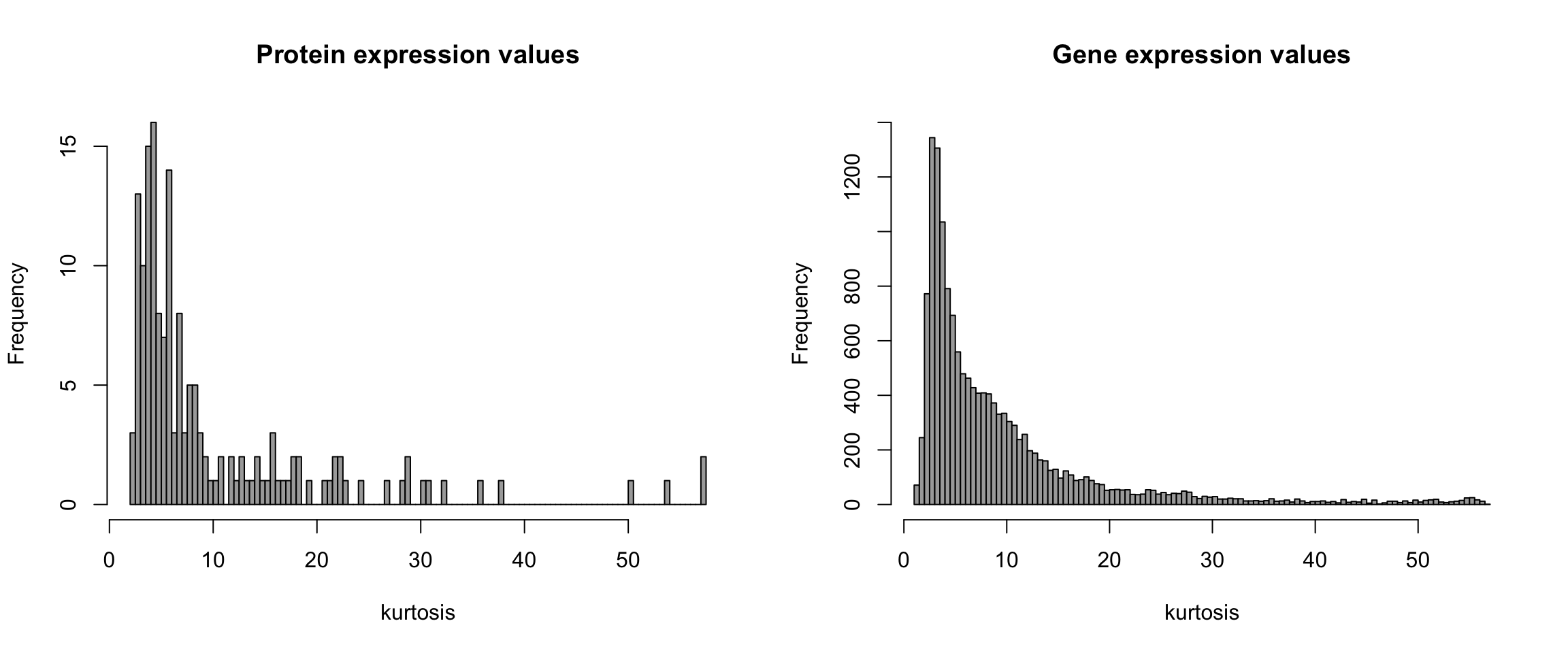
Check which one of the proteins has the highest variance:
KRT19_protein$Gene.name.d[which.max(
      apply(2^KRT19_protein[,7:66], function(x) sd(x), MAR = 1))]
[1] "KRT19"This will be our outcome.
Merge gene expression and protein data
library(data.table)

# transpose data and take care of names
NCI60 <- as.data.frame(NCI60_new)
NCI60$Gene.name.d <- rownames(NCI60_new)
NCI60t <- transpose(NCI60)
colnames(NCI60t) <- rownames(NCI60)
rownames(NCI60t) <- colnames(NCI60)
rm(NCI60_new)

# get the right protein values
KRT19_protein_n <- KRT19_protein[KRT19_protein$Gene.name.d == "KRT19",c(7:66)]
KRT19_protein_n <- KRT19_protein_n[,names(KRT19_protein_n) %in% names(NCI60)]

# Add the Protein to the gene expression
NCI60 <- NCI60t[1:59,]
NCI60[,1] <- as.numeric(2^KRT19_protein_n[,rownames(NCI60)])
names(NCI60)[1] <-  "KRT19_protein"
NCI60 <- data.frame(apply(NCI60, 2, function(x) as.numeric(x)))
rm(KRT19_protein, KRT19_protein_n)
Figure 7.8: Histogram and density of outcome
hist(NCI60$KRT19_protein, breaks = 100, prob = TRUE, col = "darkgrey",
     xlab ="KRT 19 protein", main = "", las = 1)
lines(density(NCI60$KRT19_protein), lwd = 2)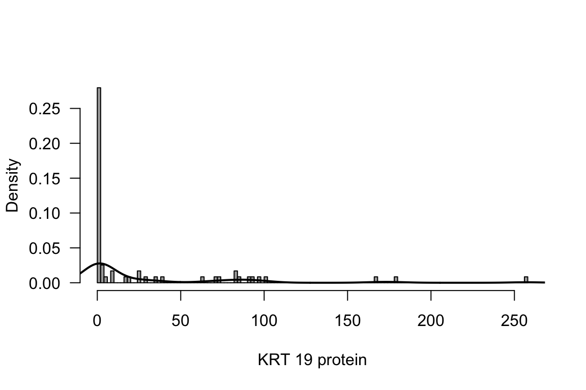
Model fitting
Choose suitable distribution
gam1 <- gamlss(KRT19_protein ~ KRT19, data = NCI60,
               sigma.formula = ~ KRT19,
               nu.formula = ~ KRT19 ,
               tau.formula = ~ KRT19)
GAMLSS-RS iteration 1: Global Deviance = 453.2066
GAMLSS-RS iteration 2: Global Deviance = 422.2179
GAMLSS-RS iteration 3: Global Deviance = 420.2152
GAMLSS-RS iteration 4: Global Deviance = 420.1806
GAMLSS-RS iteration 5: Global Deviance = 420.1802 findD <- chooseDist(gam1, type = "realplus")minimum GAIC(k= 2 ) family: GG
minimum GAIC(k= 3.84 ) family: GG
minimum GAIC(k= 4.08 ) family: GG Function to run boosting with leave-one-out CV
AMP <- function(i){
  # for reproducibility
  set.seed(i)
  # just for information
  print(i)

  # fit initial model without observation i
   glm1 <- glmboostLSS( KRT19_protein ~ .,
                        data = NCI60[-i,],
                        control = boost_control(mstop=1, nu = 0.01),
                        method = "noncyclic", families = as.families("GG"))
  # 25-fold subsampling to determine mstop
  cvrisk_glm1 <- cvrisk(folds = cv(weights = model.weights(glm1),
                                   type = "subsampling"),
                        glm1, grid = 1:150, papply = lapply)
  # set mstop to the 'optimal' value
  mstop(glm1) <- mstop(cvrisk_glm1)

  # compute prediction on oobag obs
  preds <- predict(glm1, type = "response", newdata = data_set[i,])

  return(c(mu = preds$mu, sigma = preds$sigma, nu = preds$nu,
           mstop = mstop(cvrisk_glm1),
           sel_mu = length(coef(glm1$mu)),
           sel_sigma = length(coef(glm1$sigma)),
           sel_nu = length(coef(glm1$nu))))
}
Run in parallel on multiple cores (Linux environment, takes some time…)
library(parallel)
i <- 1:nrow(data_set) # each observation one i
ERG <- mclapply(i, FUN = AMP, mc.cores = 5, mc.preschedule = FALSE)
Check how many genes were selected
# For the mu parameter
summary(unlist(lapply(ERG, function(x) x[5])))
Min. 1st Qu. Median Mean 3rd Qu. Max.
0.000 2.000 3.000 2.475 3.500 6.000 # for sigma
summary(unlist(lapply(ERG, function(x) x[6]))) Min. 1st Qu. Median Mean 3rd Qu. Max.
1.00 10.00 12.00 10.76 14.50 18.00 # for nu
table(unlist(lapply(ERG, function(x) x[7])))
 0  2
58  1
References
Sun, Qiang, Wen-Xin Zhou, and Jianqing Fan. 2020. “Adaptive Huber Regression.” Journal of the American Statistical Association 115 (529): 254–65.